ANNEX I

A.4.	VAPOUR PRESSURE

1.   METHOD

This method is equivalent to OECD TG 104 (2004).

1.1.   INTRODUCTION

This revised version of method A.4(1) includes one additional method; Effusion method: isothermal thermogravimetry, designed for substances with very low pressures (down to 10–10 Pa). In the light of needs for procedures, especially in relation to obtaining vapour pressure for substances with low vapour pressure, other procedures of this method are re-evaluated with respect to other applicability ranges.

At the thermodynamic equilibrium the vapour pressure of a pure substance is a function of temperature only. The fundamental principles are described elsewhere (2)(3).

No single measurement procedure is applicable to the entire range of vapour pressures from less than 10–10 to 105 Pa. Eight methods for measuring vapour pressure are included in this method which can be applied in different vapour pressure ranges. The various methods are compared as to application and measuring range in Table 1. The methods can only be applied for compounds that do not decompose under the conditions of the test. In cases where the experimental methods cannot be applied due to technical reasons, the vapour pressure can also be estimated, and a recommended estimation method is set out in the Appendix.

1.2.   DEFINITIONS AND UNITS

The vapour pressure of a substance is defined as the saturation pressure above a solid or liquid substance.

The SI unit of pressure, which is the pascal (Pa), should be used. Other units which have been employed historically are given hereafter, together with their conversion factors:

1 Torr	=	1 mm Hg	=	1,333 × 102 Pa
1 atmosphere	=	1,013 × 105 Pa
1 bar	=	105 Pa

The SI unit of temperature is the kelvin (K). The conversion of degrees Celsius to kelvin is according to the formula:

T = t + 273,15

where, T is the kelvin or thermodynamic temperature and t is the Celsius temperature.

Table 1

Measuring method	Substances		Estimated repeatability	Estimated reproducibility	Recommended range
	Solid	Liquid
Dynamic method	Low melting	Yes	up to 25 % 1 to 5 %	up to 25 % 1 to 5 %	103 Pa to 2 × 103 Pa 2 × 103 Pa to 105 Pa
Static method	Yes	Yes	5 to 10 %	5 to 10 %	10 Pa to 105 Pa 10–2 Pa to 105 Pa (1)
Isoteniscope method	Yes	Yes	5 to 10 %	5 to 10 %	102 Pa to 105 Pa
Effusion method: vapour pressure balance	Yes	Yes	5 to 20 %	up to 50 %	10–3 to 1 Pa
Effusion method: Knudsen cell	Yes	Yes	10 to 30 %	—	10–10 to 1 P
Effusion method: isothermal thermogravimetry	Yes	Yes	5 to 30 %	up to 50 %	10–10 to 1 Pa
Gas saturation method	Yes	Yes	10 to 30 %	up to 50 %	10–10 to 103 Pa
Spinning rotor method	Yes	Yes	10 to 20 %	—	10–4 to 0,5 Pa

1.3.   PRINCIPLE OF THE TEST

In general, the vapour pressure is determined at various temperatures. In a limited temperature range, the logarithm of the vapour pressure of a pure substance is a linear function of the inverse of the thermodynamic temperature according to the simplified Clapeyron-Clausius equation:

where:

p	=	the vapour pressure in pascals
ΔHv	=	the heat of vaporisation in J mol–1
R	=	the universal gas constant, 8,314 J mol–1 K–1
T	=	the temperature in K

1.4.   REFERENCE SUBSTANCES

Reference substances do not need to be employed. They serve primarily to check the performance of a method from time to time as well as to allow comparison between results of different methods.

1.5.   DESCRIPTION OF THE METHOD

1.5.1.   Dynamic method (Cottrell’s method)

1.5.1.1.   Principle

The vapour pressure is determined by measuring the boiling temperature of the substance at various specified pressures between roughly 103 and 105 Pa. This method is also recommended for the determination of the boiling temperature. For that purpose it is useful up to 600 K. The boiling temperatures of liquids are approximately 0,1 °C higher at a depth of 3 to 4 cm than at the surface because of the hydrostatic pressure of the column of liquid. In Cottrell’s method (4) the thermometer is placed in the vapour above the surface of the liquid and the boiling liquid is made to pump itself continuously over the bulb of the thermometer. A thin layer of liquid which is in equilibrium with vapour at atmospheric pressure covers the bulb. The thermometer thus reads the true boiling point, without errors due to superheating or hydrostatic pressure. The pump originally employed by Cottrell is shown in figure 1. Tube A contains the boiling liquid. A platinum wire B sealed into the bottom facilitates uniform boiling. The side tube C leads to a condenser, and the sheath D prevents the cold condensate from reaching the thermometer E. When the liquid in A is boiling, bubbles and liquid trapped by the funnel are poured via the two arms of the pump F over the bulb of the thermometer.

Figure 1

Figure 2

Cottrell pump (4)

A:	Thermocouple

B:	Vacuum buffer volume

C:	Pressure gauge

D:

Vacuum

E:	Measuring point

F:	Heating element c.a. 150 W

1.5.1.2.   Apparatus

A very accurate apparatus, employing the Cottrell principle, is shown in figure 2. It consists of a tube with a boiling section in the lower part, a cooler in the middle part, and an outlet and flange in the upper part. The Cottrell pump is placed in the boiling section which is heated by means of an electrical cartridge. The temperature is measured by a jacketed thermocouple, or resistance thermometer inserting through the flange at the top. The outlet is connected to the pressure regulation system. The latter consists of a vacuum pump, a buffer volume, a manostat for admitting nitrogen for pressure regulation and manometer.

1.5.1.3.   Procedure

The substance is placed in the boiling section. Problems may be encountered with non-powder solids but these can sometimes be solved by heating the cooling jacket. The apparatus is sealed at the flange and the substance degassed. Frothing substances cannot be measured using this method.

The lowest desired pressure is then set and the heating is switched on. At the same time, the temperature sensor is connected to a recorder.

Equilibrium is reached when a constant boiling temperature is recorded at constant pressure. Particular care must be taken to avoid bumping during boiling. In addition, complete condensation must occur on the cooler. When determining the vapour pressure of low melting solids, care should be taken to prevent the condenser from blocking.

After recording this equilibrium point, a higher pressure is set. The process is continued in this manner until 105 Pa has been reached (approximately 5 to 10 measuring points in all). As a check, equilibrium points must be repeated at decreasing pressures.

1.5.2.   Static method

1.5.2.1.   Principle

In the static method (5), the vapour pressure at thermodynamic equilibrium is determined at a specified temperature. This method is suitable for substances and multicomponent liquids and solids in the range from 10–1 to 105 Pa and, provided care is taken, also in the range 1 to 10 Pa.

1.5.2.2.   Apparatus

The equipment consists of a constant-temperature bath (precision of ±0,2 K), a container for the sample connected to a vacuum line, a manometer and a system to regulate the pressure. The sample chamber (figure 3a) is connected to the vacuum line via a valve and a differential manometer (U-tube containing a suitable manometer fluid) which serves as zero indicator. Mercury, silicones and phthalates are suitable for use in the differential manometer, depending on the pressure range and the chemical behaviour of the test substance. However, based on environmental concerns, the use of mercury should be avoided, if possible. The test substance must not dissolve noticeably in, or react with, the U-tube fluid. A pressure gauge can be used instead of a U-tube (figure 3b). For the manometer, mercury can be used in the range from normal pressure down to 102 Pa, while silicone fluids and phthalates are suitable for use below 102 Pa down to 10 Pa. There are other pressure gauges which can be used below 102 Pa and heatable membrane capacity manometers can even be used at below 10–1 Pa. The temperature is measured on the outside wall of the vessel containing the sample or in the vessel itself.

1.5.2.3.   Procedure

Using the apparatus as described in figure 3a, fill the U-tube with the chosen liquid, which must be degassed at an elevated temperature before readings are taken. The test substance is placed in the apparatus and degassed at reduced temperature. In the case of a multiple-component sample, the temperature should be low enough to ensure that the composition of the material is not altered. Equilibrium can be established more quickly by stirring. The sample can be cooled with liquid nitrogen or dry ice, but care should be taken to avoid condensation of air or pump-fluid. With the valve over the sample vessel open, suction is applied for several minutes to remove the air. If necessary, the degassing operation is repeated several times.

Figure 3a

Figure 3b

When the sample is heated with the valve closed, the vapour pressure increases. This alters the equilibrium of the fluid in the U-tube. To compensate for this, nitrogen or air is admitted to the apparatus until the differential pressure indicator is at zero again. The pressure required for this can be read off the manometer or off an instrument of higher precision. This pressure corresponds to the vapour pressure of the substance at the temperature of the measurement. Using the apparatus described in figure 3b, the vapour pressure is read off directly.

The vapour pressure is determined at suitably small temperature intervals (approximately 5 to 10 measuring points in all) up to the desired temperature maximum.

Low-temperature readings must be repeated as a check. If the values obtained from the repeated readings do not coincide with the curve obtained for increasing temperature, this may be due to one of the following situations:

(i)	the sample still contains air (e.g. in the case of highly viscous materials) or low-boiling substances which is or are released during heating;

(ii)	the substance undergoes a chemical reaction in the temperature range investigated (e.g. decomposition, polymerisation).

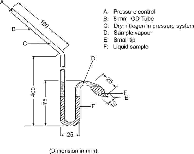
1.5.3.   Isoteniscope Method

1.5.3.1.   Principle

The isoteniscope (6) is based on the principle of the static method. The method involves placing a sample in a bulb maintained at constant temperature and connected to a manometer and a vacuum pump. Impurities more volatile than the substance are removed by degassing at reduced pressure. The vapour pressure of the sample at selected temperatures is balanced by a known pressure of inert gas. The isoteniscope was developed to measure the vapour pressure of certain liquid hydrocarbons but it is appropriate for the investigation of solids as well. The method is usually not suitable for multicomponent systems. Results are subject to only slight errors for samples containing non-volatile impurities. The recommended range is 102 to 105 Pa.

1.5.3.2.   Apparatus

An example of a measuring device is shown in figure 4. A complete description can be found in ASTM D 2879-86 (6).

1.5.3.3.   Procedure

In the case of liquids, the substance itself serves as the fluid in the differential manometer. A quantity of the liquid, sufficient to fill the bulb and the short leg of the manometer, is put in the isoteniscope. The isoteniscope is attached to a vacuum system and evacuated, then filled by nitrogen. The evacuation and purge of the system is repeated twice to remove residual oxygen. The filled isoteniscope is placed in a horizontal position so that the sample spreads out into a thin layer in the sample bulb and manometer. The pressure of the system is reduced to 133 Pa and the sample is gently warmed until it just boils (removal of dissolved gases). The isoteniscope is then placed so that the sample returns to the bulb and fills the short leg of the manometer. The pressure is maintained at 133 Pa. The drawn-out tip of the sample bulb is heated with a small flame until the sample vapour released expands sufficiently to displace part of the sample from the upper part of the bulb and manometer arm into the manometer, creating a vapour-filled, nitrogen-free space. The isoteniscope is then placed in a constant temperature bath, and the pressure of the nitrogen is adjusted until it equals that of the sample. At the equilibrium, the pressure of the nitrogen equals the vapour pressure of the substance.

Figure 4

In the case of solids, and depending on the pressure and temperature ranges, manometer liquids such as silicon fluids or phthalates are used. The degassed manometer liquid is put in a bulge provided on the long arm of the isoteniscope. Then the solid to be investigated is placed in the sample bulb and is degassed at an elevated temperature. After that, the isoteniscope is inclined so that the manometer liquid can flow into the U-tube.

1.5.4.   Effusion method: vapour pressure balance (7)

1.5.4.1.   Principle

A sample of the test substance is heated in a small furnace and placed in an evacuated bell jar. The furnace is covered by a lid which carries small holes of known diameters. The vapour of the substance, escaping through one of the holes, is directed onto a balance pan of a highly sensitive balance which is also enclosed in the evacuated bell jar. In some designs the balance pan is surrounded by a refrigeration box, providing heat dissipation to the outside by thermal conduction, and is cooled by radiation so that the escaping vapour condenses on it. The momentum of the vapour jet acts as a force on the balance. The vapour pressure can be derived in two ways: directly from the force on the balance pan and also from the evaporation rate using the Hertz-Knudsen equation (2):

where:

G	=	evaporation rate (kg s–1 m–2)
M	=	molar mass (g mol–1)
T	=	temperature (K)
R	=	universal gas constant (J mol–1 K–1)
P	=	vapour pressure (Pa)

The recommended range is 10–3 to 1 Pa.

1.5.4.2.   Apparatus

The general principle of the apparatus is illustrated in figure 5.

Figure 5

A:	Base plate	F:	Refrigeration box and cooling bar
B:	Moving coil instrument	G:	Evaporator furnace
C:	Bell jar	H:	Dewar flask with liquid nitrogen
D:	Balance with scale pan	I:	Measurement of temperature of sample
E:	Vacuum measuring device	J:	Test Substance

1.5.5.   Effusion method: Knudsen cell

1.5.5.1.   Principle

The method is based on the estimation of the mass of test substance flowing out per unit of time of a Knudsen cell (8) in the form of vapour, through a micro-orifice under ultra-vacuum conditions. The mass of effused vapour can be obtained either by determining the loss of mass of the cell or by condensing the vapour at low temperature and determining the amount of volatilised substance using chromatography. The vapour pressure is calculated by applying the Hertz-Knudsen relation (see section 1.5.4.1) with correction factors that depend on parameters of the apparatus (9). The recommended range is 10–10 to 1 Pa (10)(11)(12)(13)(14).

1.5.5.2.   Apparatus

The general principle of the apparatus is illustrated in figure 6.

Figure 6

1:	Connection to vacuum	7:	Threaded lid
2:	Wells from platinum resistance thermometer or temperature measurement and control	8:	Butterfly nuts
3:	Lid for vacuum tank	9:	Bolts
4:	O-ring	10:	Stainless steel effusion cells
5:	Aluminum vacuum tank	11:	Heater cartridge
6:	Device for installing and removing the effusion cells

1.5.6.   Effusion method: isothermal thermogravimetry

1.5.6.1.   Principle

The method is based on the determination of accelerated evaporation rates for the test substance at elevated temperatures and ambient pressure using thermogravimetry (10)(15)(16)(17)(18)(19)(20). The evaporation rates vT result from exposing the selected compound to a slowly flowing inert gas atmosphere, and monitoring the weight loss at defined isothermal temperatures T in Kelvin over appropriate periods of time. The vapour pressures pT are calculated from the vT values by using the linear relationship between the logarithm of the vapour pressure and the logarithm of the evaporation rate. If necessary, an extrapolation to temperatures of 20 and 25 °C can be made by regression analysis of log pT vs. 1/T. This method is suitable for substances with vapour pressures as low as 10–10 Pa (10–12 mbar) and with purity as close as possible to 100 % to avoid the misinterpretation of measured weight losses.

1.5.6.2.   Apparatus

The general principle of the experimental set-up is shown in figure 7.

Figure 7

The sample carrier plate, hanging on a microbalance in a temperature controlled chamber, is swept by a stream of dry nitrogen gas which carries the vaporised molecules of the test substance away. After leaving the chamber, the gas stream is purified by a sorption unit.

1.5.6.3.   Procedure

The test substance is applied to the surface of a roughened glass plate as a homogeneous layer. In the case of solids, the plate is wetted uniformly by a solution of the substance in a suitable solvent and dried in an inert atmosphere. For the measurement, the coated plate is hung into the thermogravimetric analyser and subsequently its weight loss is measured continuously as a function of time.

The evaporation rate vT at a definite temperature is calculated from the weight loss Δm of the sample plate by

where F is the surface area of the coated test substances, normally the surface area of the sample plate, and t is the time for weight loss Δm.

The vapour pressure pT is calculated on the basis of its function of evaporation rate vT:

Log pT = C + D · log vT

where C and D are constants specific for the experimental arrangement used, depending on the diameter of the measurement chamber and on the gas flow rate. These constants must be determined once by measuring a set of compounds with known vapour pressure and regressing log pT vs. log vT (11)(21)(22).

The relationship between the vapour pressure pT and the temperature T in Kelvin is given by

Log pT = A + B · 1/T

where A and B are constants obtained by regressing log pT vs. 1/T. With this equation, the vapour pressure can be calculated for any other temperature by extrapolation.

1.5.7.   Gas saturation method (23)

1.5.7.1.   Principle

Inert gas is passed, at room temperature and at a known flow rate, through or over a sample of the test substance, slowly enough to ensure saturation. Achieving saturation in the gas phase is of critical importance. The transported substance is trapped, generally using a sorbent, and its amount is determined. As an alternative to vapour trapping and subsequent analysis, in-train analytical techniques, like gas chromatography, may be used to determine quantitatively the amount of material transported. The vapour pressure is calculated on the assumption that the ideal gas law is obeyed and that the total pressure of a mixture of gases is equal to the sum of the pressures of the component gases. The partial pressure of the test substance, i.e. the vapour pressure, is calculated from the known total gas volume and from the weight of the material transported.

The gas saturation procedure is applicable to solid or liquid substances. It can be used for vapour pressures down to 10–10 Pa (10)(11)(12)(13)(14). The method is most reliable for vapour pressures below 103 Pa. Above 103 Pa, the vapour pressures are generally overestimated, probably due to aerosol formation. Since the vapour pressure measurements are made at room temperature, the need to extrapolate data from high temperatures is not necessary and high temperature extrapolation, which can often cause serious errors, is avoided.

1.5.7.2.   Apparatus

The procedure requires the use of a constant-temperature box. The sketch in figure 8 shows a box containing three solid and three liquid sample holders, which allow for the triplicate analysis of either a solid or a liquid sample. The temperature is controlled to ±0,5 °C or better.

Figure 8

In general, nitrogen is used as an inert carrier gas but, occasionally, another gas may be required (24). The carrier gas must be dry. The gas stream is split into 6 streams, controlled by needle valves (approximately 0,79 mm orifice), and flows into the box via 3,8 mm i.d. copper tubing. After temperature equilibration, the gas flows through the sample and the sorbent trap and exists from the box.

Solid samples are loaded into 5 mm i.d. glass tubing between glass wool plugs (see Figure 9). Figure 10 shows a liquid sample holder and sorbent system. The most reproducible method for measuring the vapour pressure of liquids is to coat the liquid on glass beads or on an inert sorbent such as silica, and to pack the holder with these beads. As an alternative, the carrier gas may be made to pass a coarse frit and bubble through a column of the liquid test substance.

Figure 9

Figure 10

The sorbent system contains a front and a backup sorbent section. At very low vapour pressures, only small amounts are retained by the sorbent and the adsorption on the glass wool and the glass tubing between the sample and the sorbent may be a serious problem.

Traps cooled with solid CO2 are another efficient way for collecting the vaporised material. They do not cause any back pressure on the saturator column and it is also easy to quantitatively remove the trapped material.

1.5.7.3.   Procedure

The flow rate of the effluent carrier gas is measured at room temperature. The flow rate is checked frequently during the experiment to assure that there is an accurate value for the total volume of carrier gas. Continuous monitoring with a mass flow-meter is preferred. Saturation of the gas phase may require considerable contact time and hence quite low gas flow rates (25).

At the end of the experiment, both the front and backup sorbent sections are analysed separately. The compound on each section is desorbed by adding a solvent. The resulting solutions are analysed quantitatively to determine the weight desorbed from each section. The choice of the analytical method (also the choice of sorbent and desorbing solvent) is dictated by the nature of the test material. The desorption efficiency is determined by injecting a known amount of sample onto the sorbent, desorbing it and analysing the amount recovered. It is important to check the desorption efficiency at or near the concentration of the sample under the test conditions.

To assure that the carrier gas is saturated with the test substance, three different gas flow rates are used. If the calculated vapour pressure shows no dependence on flow rate, the gas is assumed to be saturated.

The vapour pressure is calculated through the equation:

where:

p	=	vapour pressure (Pa)
W	=	mass of evaporated test substance (g)
V	=	volume of saturated gas (m3)
R	=	universal gas constant 8,314 (J mol–1 K–1)
T	=	temperature (K)
M	=	molar mass of test substance (g mol–1)

Measured volumes must be corrected for pressure and temperature differences between the flow meter and the saturator.

1.5.8.   Spinning rotor

1.5.8.1.   Principle

This method uses a spinning rotor viscosity gauge, in which the measuring element is a small steel ball which, suspended in a magnetic field, is made to spin by rotating fields (26)(27)(28). Pick-up coils allow its spinning rate to be measured. When the ball has reached a given rotational speed, usually about 400 revolutions per second, energising is stopped and deceleration, due to gas friction, takes place. The drop of rotational speed is measured as a function of time. The vapour pressure is deduced from the pressure-dependent slow-down of the steel ball. The recommended range is 10–4 to 0,5 Pa.

1.5.8.2.   Apparatus

A schematic drawing of the experimental set-up is shown in figure 11. The measuring head is placed in a constant-temperature enclosure, regulated within 0,1 °C. The sample container is placed in a separate enclosure, also regulated within 0,1 °C. All other parts of the set-up are kept at a higher temperature to prevent condensation. The whole apparatus is connected to a high-vacuum system.

Figure 11

2.   DATA AND REPORTING

2.1.   DATA

The vapour pressure from any of the preceding methods should be determined for at least two temperatures. Three or more are preferred in the range from 0 to 50 °C, in order to check the linearity of the vapour pressure curve. In case of Effusion method (Knudsen cell and isothermal thermogravimetry) and Gas saturation method, 120 to 150 °C is recommended for the measuring temperature range instead of 0 to 50 °C.

2.2.   TEST REPORT

The test report must include the following information:

—	method used,

—	precise specification of the substance (identity and impurities) and preliminary purification step, if any,

—	at least two vapour pressure and temperature values — and preferably three or more — required in the range from 0 to 50 °C (or 120 to 150 °C),

—	at least one of the temperatures should be at or below 25 °C, if technically possible according to the chosen method,

—	all original data,

—	a log p versus 1/T curve,

—	an estimate of the vapour pressure at 20 or 25 °C.

If a transition (change of state, decomposition) is observed, the following information should be noted:

—	nature of the change,

—	temperature at which the change occurs at atmospheric pressure,

—	vapour pressure at 10 and 20 °C below the transition temperature and 10 and 20 °C above this temperature (unless the transition is from solid to gas).

All information and remarks relevant for the interpretation of results have to be reported, especially with regard to impurities and physical state of the substance.

3.   LITERATURE

(1)	Official Journal of the European Communities L 383 A, 26-47 (1992).

(2)	Ambrose, D. (1975). Experimental Thermodynamics, Vol. II, Le Neindre, B., and Vodar, B., Eds., Butterworths, London.

(3)	Weissberger R., ed. (1959). Technique of Organic Chemistry, Physical Methods of Organic Chemistry, 3rd ed., Vol. I, Part I. Chapter IX, Interscience Publ., New York.

(4)	Glasstone, S. (1946). Textbook of Physical Chemistry, 2nd ed., Van Nostrand Company, New York.

(5)	NF T 20-048 AFNOR (September 1985). Chemical products for industrial use — Determination of vapour pressure of solids and liquids within a range from 10–1 to 105 Pa — Static method.

(6)	ASTM D 2879-86, Standard test method for vapour pressure — temperature relationship and initial decomposition temperature of liquids by isoteniscope.

(7)	NF T 20-047 AFNOR (September 1985). Chemical products for industrial use — Determination of vapour pressure of solids and liquids within range from 10–3 to 1 Pa — Vapour pressure balance method.

(8)	Knudsen, M. (1909). Ann. Phys. Lpz., 29, 1979; (1911), 34, 593.

(9)	Ambrose, D., Lawrenson, I.J., Sprake, C.H.S. (1975). J. Chem. Thermodynamics 7, 1173.

(10)	Schmuckler, M.E., Barefoot, A.C., Kleier, D.A., Cobranchi, D.P. (2000), Vapor pressures of sulfonylurea herbicides; Pest Management Science 56, 521-532.

(11)	Tomlin, C.D.S. (ed.), The Pesticide Manual, Twelfth Edition (2000).

(12)	Friedrich, K., Stammbach, K., Gas chromatographic determination of small vapour pressures determination of the vapour pressures of some triazine herbicides. J. Chromatog. 16 (1964), 22-28.

(13)	Grayson, B.T., Fosbraey, L.A., Pesticide Science 16 (1982), 269-278.

(14)	Rordorf, B.F., Prediction of vapor pressures, boiling points and enthalpies of fusion for twenty-nine halogenated dibenzo-p-dioxins, Thermochimia Acta 112 Issue 1 (1987), 117-122.

(15)	Gückel, W., Synnatschke, G., Ritttig, R., A Method for Determining the Volatility of Active Ingredients Used in Plant Protection; Pesticide Science 4 (1973) 137-147.

(16)	Gückel, W., Synnatschke, G., Ritttig, R., A Method for Determining the Volatility of Active Ingredients Used in Plant Protection II. Application to Formulated Products; Pesticide Science 5 (1974) 393-400.

(17)	Gückel, W., Kaestel, R., Lewerenz, J., Synnatschke, G., A Method for Determining the Volatility of Active Ingredients Used in Plant Protection. Part III: The Temperature Relationship between Vapour Pressure and Evaporation Rate; Pesticide Science 13 (1982) 161-168.

(18)	Gückel, W., Kaestel, R., Kroehl, T., Parg, A., Methods for Determining the Vapour Pressure of Active Ingredients Used in Crop Protection. Part IV: An Improved Thermogravimetric Determination Based on Evaporation Rate; Pesticide Science 45 (1995) 27-31.

(19)	Kroehl, T., Kaestel, R., Koenig, W., Ziegler, H., Koehle, H., Parg, A., Methods for Determining the Vapour Pressure of Active Ingredients Used in Crop Protection. Part V: Thermogravimetry Combined with Solid Phase MicroExtraction (SPME); Pesticide Science, 53 (1998) 300-310.

(20)	Tesconi, M., Yalkowsky, S.H., A Novel Thermogravimetric Method for Estimating the Saturated Vapor Pressure of Low-Volatility Compounds; Journal of Pharmaceutical Science 87(12) (1998) 1512-20.

(21)	Lide, D.R. (ed.), CRC Handbook of Chemistry and Physics, 81st ed. (2000), Vapour Pressure in the Range — 25 °C to 150 °C.

(22)	Meister, R.T. (ed.), Farm Chemicals Handbook, Vol. 88 (2002).

(23)	40 CFR, 796. (1993). pp 148-153, Office of the Federal Register, Washington DC.

(24)	Rordorf B.F. (1985). Thermochimica Acta 85, 435.

(25)	Westcott et al. (1981). Environ. Sci. Technol. 15, 1375.

(26)	Messer G., Röhl, P., Grosse G., and Jitschin W. (1987). J. Vac. Sci. Technol. (A), 5(4), 2440.

(27)	Comsa G., Fremerey J.K., and Lindenau, B. (1980). J. Vac. Sci. Technol. 17(2), 642.

(28)	Fremerey, J.K. (1985). J. Vac. Sci. Technol. (A), 3(3), 1715.

---

(1)  When using a capacitance manometer

ANNEX II

A.22.

LENGTH WEIGHTED GEOMETRIC MEAN DIAMETER OF FIBRES

1.   METHOD

1.1.   INTRODUCTION

This method describes a procedure to measure the Length Weighted Geometric Mean Diameter (LWGMD) of bulk Man Made Mineral Fibres (MMMF). As the LWGMD of the population will have a 95 % probability of being between the 95 % confidence levels (LWGMD ± two standard errors) of the sample, the value reported (the test value) will be the lower 95 % confidence limit of the sample (i.e. LWGMD — 2 standard errors). The method is based on an update (June 1994) of a draft HSE industry procedure agreed at a meeting between ECFIA and HSE at Chester on 26/9/93 and developed for and from a second inter-laboratory trial (1, 2). This measurement method can be used to characterise the fibre diameter of bulk substances or products containing MMMFs including refractory ceramic fibres (RCF), man-made vitreous fibres (MMVF), crystalline and polycrystalline fibres.

Length weighting is a means of compensating for the effect on the diameter distribution caused by the breakage of long fibres when sampling or handling the material. Geometric statistics (geometric mean) are used to measure the size distribution of MMMF diameters because these diameters usually have size distributions that approximate to log normal.

Measuring length as well as diameter is both tedious and time consuming but, if only those fibres that touch an infinitely thin line on a SEM field of view are measured, then the probability of selecting a given fibre is proportional to its length. As this takes care of the length in the length weighting calculations, the only measurement required is the diameter and the LWGMD-2SE can be calculated as described.

1.2.   DEFINITIONS

Particle: An object with a length to width ratio of less than 3:1.

Fibre: An object with a length to with ratio (aspect ratio) of at least 3:1.

1.3.   SCOPE AND LIMITATIONS

The method is designed to look at diameter distributions which have median diameters from 0,5 μm to 6 μm. Larger diameters can be measured by using lower SEM magnifications but the method will be increasingly limited for finer fibre distributions and a TEM (transmission electron microscope) measurement is recommended if the median diameter is below 0,5 μm.

1.4.   PRINCIPLE OF THE TEST METHOD

A number of representative core samples are taken from the fibre blanket or from loose bulk fibre. The bulk fibres are reduced in length using a crushing procedure and a representative sub-sample dispersed in water. Aliquots are extracted and filtered through a 0,2 μm pore size, polycarbonate filter and prepared for examination using scanning electron microscope (SEM) techniques. The fibre diameters are measured at a screen magnification of × 10 000 or greater (1) using a line intercept method to give an unbiased estimate of the median diameter. The lower 95 % confidence interval (based on a one sided test) is calculated to give an estimate of the lowest value of the geometric mean fibre diameter of the material.

1.5.   DESCRIPTION OF THE TEST METHOD

1.5.1.   Safety/precautions

Personal exposure to airborne fibres should be minimised and a fume cupboard or glove box should be used for handling the dry fibres. Periodic personal exposure monitoring should be carried out to determine the effectiveness of the control methods. When handling MMMF’s disposable gloves should be worn to reduce skin irritation and to prevent cross-contamination.

1.5.2.   Apparatus/equipment

—	Press and dyes (capable of producing 10 MPa).

—	0,2 μm pore size polycarbonate capillary pore filters (25 mm diameter).

—	5 μm pore size cellulose ester membrane filter for use as a backing filter.

—	Glass filtration apparatus (or disposable filtration systems) to take 25 mm diameter filters (e.g. Millipore glass microanalysis kit, type No XX10 025 00).

—	Freshly distilled water that has been filtered through a 0,2 μm pore size filter to remove micro-organisms.

—	Sputter coater with a gold or gold/palladium target.

—	Scanning electron microscope capable of resolving down to 10 nm and operating at × 10 000 magnification.

—	Miscellaneous: spatulas, type 24 scalpel blade, tweezers, SEM tubes, carbon glue or carbon adhesive tape, silver dag.

—	Ultrasonic probe or bench top ultrasonic bath.

—	Core sampler or cork borer, for taking core samples from MMMF blanket.

1.5.3.   Test Procedure

1.5.3.1.   Sampling

For blankets and bats a 25 mm core sampler or cork borer is used to take samples of the cross-section. These should be equally spaced across the width of a small length of the blanket or taken from random areas if long lengths of the blanket are available. The same equipment can be used to extract random samples from loose fibre. Six samples should be taken when possible, to reflect spatial variations in the bulk material.

The six core samples should be crushed in a 50 mm diameter dye at 10 MPa. The material is mixed with spatula and re-pressed at 10 MPa. The material is then removed from the dye and stored in a sealed glass bottle.

1.5.3.2.   Sample Preparation

If necessary, organic binder can be removed by placing the fibre inside a furnace at 450 °C for about one hour.

Cone and quarter to subdivide the sample (this should be done inside a dust cupboard).

Using a spatula, add a small amount (< 0,5 g) of sample to 100 ml of freshly distilled water that has been filtered through a 0,2 μm membrane filter (alternative sources of ultra pure water may be used if they are shown to be satisfactory). Disperse thoroughly by the use of an ultrasonic probe operated at 100 W power and tuned so that cavitation occurs. (If a probe is not available use the following method: repeatedly shake and invert for 30 seconds; ultrasonic in a bench top ultrasonic bath for five minutes; then repeatedly shake and invert for a further 30 seconds.)

Immediately after dispersion of the fibre, remove a number of aliquots (e.g. three aliquots of 3, 6 and 10 ml) using a wide-mouthed pipette (2-5 ml capacity).

Vacuum filter each aliquot through a 0,2 μm polycarbonate filter supported by a 5 µm pore MEC backing filter, using a 25 mm glass filter funnel with a cylindrical reservoir. Approximately 5 ml of filtered distilled water should be placed into the funnel and the aliquot slowly pipetted into the water holding the pipette tip below the meniscus. The pipette and the reservoir must be flushed thoroughly after pipetting, as thin fibres have a tendency to be located more on the surface.

Carefully remove the filter and separate it from the backing filter before placing it in a container to dry.

Cut a quarter or half filter section of the filtered deposit with a type 24 scalpel blade using a rocking action. Carefully attach the cut section to a SEM stub using a sticky carbon tab or carbon glue. Silver dag should be applied in at least three positions to improve the electrical contact at the edges of the filter and the stub. When the glue/silver dag is dry, sputter coat approximately 50 nm of gold or gold/palladium onto the surface of the deposit.

1.5.3.3.   SEM calibration and operation

1.5.3.3.1.   Calibration

The SEM calibration should be checked at least once a week (ideally once a day) using a certified calibration grid. The calibration should be checked against a certified standard and if the measured value (SEM) is not within ±2 % of the certified value, then the SEM calibration must be adjusted and re-checked.

The SEM should be capable of resolving at least a minimum visible diameter of 0,2 µm, using a real sample matrix, at a magnification of × 2 000.

1.5.3.3.2.   Operation

The SEM should be operated at 10 000 magnification (2) using conditions that give good resolution with an acceptable image at slow scan rates of, for example, 5 seconds per frame. Although the operational requirements of different SEMs may vary, generally to obtain the best visibility and resolution, with relatively low atomic weight materials, accelerating voltages of 5-10 keV should be used with a small spot size setting and short working distance. As a linear traverse is being conducted, then a 0° tilt should be used to minimise re-focussing or, if the SEM has a eucentric stage, the eucentric working distance should be used. Lower magnification may be used if the material does not contain small (diameter) fibres and the fibre diameters are large (> 5 μm).

1.5.3.4.   Sizing

1.5.3.4.1.   Low magnification examination to assess the sample

Initially the sample should be examined at low magnification to look for evidence of clumping of large fibres and to assess the fibre density. In the event of excessive clumping it is recommended that a new sample is prepared.

For statistical accuracy it is necessary to measure a minimum number of fibres and high fibre density may seem desirable as examining empty fields is time consuming and does not contribute to the analysis. However, if the filter is overloaded, it becomes difficult to measure all the measurable fibres and, because small fibres may be obscured by larger ones, they may be missed.

Bias towards over estimating the LWGMD may result from fibre densities in excess of 150 fibres per millimetre of linear traverse. On the other hand, low fibre concentrations will increase the time of analysis and it is often cost effective to prepare a sample with a fibre density closer to the optimum than to persist with counts on low concentration filters. The optimum fibre density should give an average of about one or two countable fibre per fields of view at 5 000 magnification. Nevertheless the optimum density will depend on the size (diameter) of the fibres, so it is necessary that the operator uses some expert judgement in order to decide whether the fibre density is close to optimal or not.

1.5.3.4.2.   Length weighting of the fibre diameters

Only those fibres that touch (or cross) an (infinitely) thin line drawn on the screen of the SEM are counted. For this reason a horizontal (or vertical) line is drawn across the centre of the screen.

Alternatively a single point is placed at the centre of the screen and a continuous scan in one direction across the filter is initiated. Each fibre of aspect ratio grater than 3:1 touching or crossing this point has its diameter measured and recorded.

1.5.3.4.3.   Fibre sizing

It is recommended that a minimum of 300 fibres are measured. Each fibre is measured only once at the point of intersection with the line or point drawn on the image (or close to the point of intersection if the fibre edges are obscured). If fibres with non-uniform cross sections are encountered, a measurement representing the average diameter of the fibre should be used. Care should be taken in defining the edge and measuring the shortest distance between the fibre edges. Sizing may be done on line, or off-line on stored images or photographs. Semi-automated image measurement systems that download data directly into a spreadsheet are recommended, as they save time, eliminate transcription errors and calculations can be automated.

The ends of long fibres should be checked at low magnification to ensure that they do not curl back into the measurement field of view and are only measured once.

2.   DATA

2.1.   TREATMENT OF RESULTS

Fibre diameters do not usually have a normal distribution. However, by performing a log transformation it is possible to obtain a distribution that approximates to normal.

Calculate the arithmetic mean (mean lnD) and the standard deviation (SDlnD) of the log to base e values (lnD) of the n fibre diameters (D).

	(1)
	(2)

The standard deviation is divided by the square root of the number of measurements (n) to obtain the standard error (SElnD).

(3)

Subtract two times the standard error from the mean and calculate the exponential of this value (mean minus two standard errors) to give the geometric mean minus two geometric standard errors.

(4)

3.   REPORTING

TEST REPORT

The test report should include at least the following information:

—	The value of LWGMD-2SE.

—	Any deviations and particularly those which may have an effect on the precision or accuracy of the results with appropriate justifications.

4.   REFERENCES

1.	B. Tylee SOP MF 240. Health and Safety Executive, February 1999.

2.	G. Burdett and G. Revell. Development of a standard method to measure the length-weigthed geometric mean fibre diameter: Results of the Second inter-laboratory exchange. IR/L/MF/94/07. Project R42.75 HPD. Health and Safety Executive, Research and Laboratory Services Division, 1994.

---

(1)  This magnification value is indicated for 3 µm fibres, for 6 µm fibres a magnification of × 5 000 may be more suitable.

(2)  For 3 μm fibres, see previous note.

ANNEX III

B.46.

IN VITRO SKIN IRRITATION: RECONSTRUCTED HUMAN EPIDERMIS MODEL TEST

1.   METHOD

1.1.   INTRODUCTION

Skin irritation refers to the production of reversible damage to the skin following the application of a test substance for up to 4 hours [as defined by the United Nations (UN) Globally Harmonized System of Classification and Labelling of Chemicals (GHS)](1). This Test Method provides an in vitro procedure that, depending on information requirements, may allow determining the skin irritancy of substances as a stand-alone replacement test within a testing strategy, in a weight of evidence approach (2).

The assessment of skin irritation has typically involved the use of laboratory animals (See Method B.4)(3). In relation to animal welfare concerns, method B.4 allows for the determination of skin corrosion/irritation by applying a sequential testing strategy, using validated in vitro and ex vivo methods, thus avoiding pain and suffering of animals. Three validated in vitro Test Methods or Test Guidelines, B.40, B.40bis and TG 435 (4, 5, 6), are useful for the corrosivity part of the sequential testing strategy of B.4.

This Test Method is based on reconstructed human epidermis models, which in their overall design (the use of human derived epidermis keratinocytes as cell source, representative tissue and cytoarchitecture) closely mimic the biochemical and physiological properties of the upper parts of the human skin, i.e. the epidermis. The procedure described under this Test Method allows the hazard identification of irritant substances in accordance with UN GHS category 2. This Test Method also includes a set of performance standards for the assessment of similar and modified reconstructed human epidermis based test methods (7).

Prevalidation, optimisation and validation studies have been completed for two in vitro test methods (8, 9, 10, 11, 12, 13, 14, 15, 16, 17), commercially available as EpiSkin™ and EpiDerm™, using reconstructed human epidermis models. These references were based on R 38. Certain aspects of recalculation for the purposes of GHS are addressed in reference 25. Methods with a performance equivalent to EpiSkin™ (validated reference method 1) are recommended as a stand alone replacement test method for the rabbit in vivo test for classifying GHS category 2 irritant substances. Methods with a performance equivalent to EpiDerm™ (validated reference method 2) are only recommended as a screen test method, or as part of a sequential testing strategy in a weight of evidence approach, for classifying GHS category 2 irritant substances. Before a proposed in vitro reconstructed human epidermis model test for skin irritation can be used for regulatory purposes, its reliability, relevance (accuracy), and limitations for its proposed use should be determined to ensure that it is comparable to that of the validated reference method 1, in accordance with the performance standards set out in this Test Method (Appendix).

Two other in vitro reconstructed human epidermis test methods, have been validated in accordance with the requirements under this Test Method, and show similar results as the validated reference method 1 (18). These are the modified EpiDerm™ test method (modified reference method 2) and the SkinEthic RHE™ test method (me-too method 1).

1.2.   DEFINITIONS

The following definitions are applied within this Test Method:

Accuracy: The closeness of agreement between test method results and accepted reference values. It is a measure of test method performance and one aspect of relevance. The term is often used interchangeably with ‘concordance’ to mean the proportion of correct outcomes of a test method.

Batch control substance: Benchmark substance producing a mid-range cell viability response of the tissue.

Cell viability: Parameter measuring total activity of a cell population e.g. as ability of cellular mitochondrial dehydrogenases to reduce the vital dye MTT (3-(4,5-Dimethylthiazol-2-yl)-2,5-diphenyltetrazolium bromide, Thiazolyl blue;), which, depending on the endpoint measured and the test design used, correlates with the total number and/or vitality of living cells.

ET50 : The exposure time required to reduce cell viability by 50 % upon application of the marker substance at a specified, fixed concentration, see also IC50.

False negative rate: The proportion of all positive substances falsely identified by a test method as negative. It is one indicator of test method performance.

False positive rate: The proportion of all negative (non-active) substances that are falsely identified as positive. It is one indicator of test method performance.

Infinite dose: Amount of test substance applied to the skin exceeding the amount required to completely and uniformly cover the skin surface.

GHS (Globally Harmonized System of Classification and Labelling of Chemicals): A system proposing the classification of substances and mixtures according to standardised types and levels of physical, health and environmental hazards, and addressing corresponding communication elements, such as pictograms, signal words, hazard statements, precautionary statements and safety data sheets, so that to convey information on their adverse effects with a view to protect people (including employers, workers, transporters, consumers and emergency responders) and the environment (1) and implemented in the EU in Regulation (EC) No 1272/2008.

IC50 : The concentration at which a marker substance reduces the viability of the tissues by 50 % (IC50) after a fixed exposure time, see also ET50.

Performance standards: Standards, based on a validated reference method, that provide a basis for evaluating the comparability of a proposed test method that is mechanistically and functionally similar. Included are (I) essential test method components; (II) a minimum list of reference substances selected from among the substances used to demonstrate the acceptable performance of the validated reference method; and (III) the comparable levels of accuracy and reliability, based on what was obtained for the validated reference method, that the proposed test method should demonstrate when evaluated using the minimum list of reference substances.

Reliability: Measures of the extent that a test method can be performed reproducibly within and between laboratories over time, when performed using the same protocol. It is assessed by calculating intra- and inter-laboratory reproducibility.

Sensitivity: The proportion of all positive/active substances that are correctly classified by the test. It is a measure of accuracy for a test method that produces categorical results, and is an important consideration in assessing the relevance of a test method.

Specificity: The proportion of all negative/inactive substances that are correctly classified by the test. It is a measure of accuracy for a test method that produces categorical results and is an important consideration in assessing the relevance of a test method.

Skin irritation: The production of reversible damage to the skin following the application of a test substance for up to 4 hours. Skin irritation is a locally arising, non-immunogenic reaction, which appears shortly after stimulation (24). Its main characteristic is its reversible process involving inflammatory reactions and most of the clinical characteristic signs of irritation (erythema, oedema, itching and pain) related to an inflammatory process.

1.3.   SCOPE AND LIMITATIONS

A limitation of the reconstructed human epidermis tests falling under this Test Method is that they only classify substances as skin irritants according to UN GHS category 2. As they do not allow the classification of substances to the optional category 3 as defined in the UN GHS, all remaining substances will not be classified (no category). Depending on regulatory needs and possible future inclusion of new endpoints, improvements or development of new me-too tests, this Test Method may have to be revised.

This Test method allows the hazard identification of irritant mono-constituent substances (19), but it does not provide adequate information on skin corrosion. Gases and aerosols cannot be tested, while mixtures have not been assessed yet in a validation study.

1.4.   PRINCIPLE OF THE TEST

The test substance is applied topically to a three-dimensional reconstructed human epidermis model, comprised of normal, human-derived epidermal keratinocytes, which have been cultured to form a multilayered, highly differentiated model of the human epidermis. It consists of organised basal, spinous and granular layers, and a multilayered stratum corneum containing intercellular lamellar lipid layers arranged in patterns analogous to those found in vivo.

The principle of the reconstructed human epidermis model test is based on the premise that irritant substances are able to penetrate the stratum corneum by diffusion and are cytotoxic to the cells in the underlying layers. Cell viability is measured by dehydrogenase conversion of the vital dye MTT [3-(4,5-Dimethylthiazol-2-yl)-2,5-diphenyltetrazolium bromide, Thiazolyl blue; EINECS number 206-069-5, CAS number 298-93-1)], into a blue formazan salt that is quantitatively measured after extraction from tissues (20). Irritant substances are identified by their ability to decrease cell viability below defined threshold levels (i.e. ≤ 50 %, for UN GHS category 2 irritants). Substances that produce cell viabilities above the defined threshold level, will not be classified (i.e. > 50 %, no category).

The reconstructed human epidermis model systems may be used to test solids, liquids, semi-solids and waxes. The liquids may be aqueous or non-aqueous; solids may be soluble or insoluble in water. Whenever possible, solids should be tested as a fine powder. Since 58 carefully selected substances, representing a wide spectrum of chemical classes, were included in the validation of the reconstructed human epidermis model test systems, the methods are expected to be generally applicable across chemical classes (16). The validation includes 13 GHS Cat. 2 irritants. It should be noted that non-corrosive acids, bases, salts and other inorganic substances were not included in the validation and some known classes of organic irritants such as hydroperoxides, phenols and surfactants were not included or were only included to a limited extent.

1.5.   DEMONSTRATION OF PROFICIENCY

Prior to routine use of a validated method that adheres to this Test Method, laboratories may wish to demonstrate technical proficiency, using the ten substances recommended in Table 1. Under this Test Method, the UN GHS optional category 3 is considered as no category. For novel similar (me-too) test methods developed under this Test Method that are structurally and functionally similar to the validated reference methods or for modifications of validated methods, the performance standards described in the Appendix to this Test Method should be used to demonstrate comparable reliability and accuracy of the new test method prior to its use for regulatory testing.

Table 1

Proficiency Substances which are a subset of the Reference Substances listed in the Appendix

Substance	CAS Number	In vivo score	Physical state	GHS category
naphthalene acetic acid	86-87-3	0	S	No Cat.
isopropanol	67-63-0	0,3	L	No Cat.
methyl stearate	112-61-8	1	S	No Cat.
heptyl butyrate	5870-93-9	1,7	L	Optional Cat. 3
hexyl salicylate	6259-76-3	2	L	Optional Cat. 3
cyclamen aldehyde	103-95-7	2,3	L	Cat. 2
1-bromohexane	111-25-1	2,7	L	Cat. 2
butyl methacrylate	97-88-1	3	L	Cat. 2
1-methyl-3-phenyl-1-piperazine	5271-27-2	3,3	S	Cat. 2
Heptanal	111-71-7	4	L	Cat. 2

1.6.   DESCRIPTION OF THE METHOD

The following is a description of the components and procedures of a reconstructed human epidermis model test for skin irritation assessment. A reconstructed human epidermis model can be constructed, prepared or obtained commercially (e.g. EpiSkin™, EpiDerm™ and SkinEthic RHE™). Standard test method protocols for EpiSkin™, EpiDerm™ and SkinEthic RHE™ can be obtained at [http://ecvam.jrc.ec.europa.eu](21, 22, 23). Testing should be performed according to the following:

1.6.1.   Reconstructed Human Epidermis Model Components

1.6.1.1.   General model conditions

Normal human keratinocytes should be used to construct the epithelium. Multiple layers of viable epithelial cells (basal layer, stratum spinosum, stratum granulosum) should be present under a functional stratum corneum. Stratum corneum should be multilayered containing the essential lipid profile to produce a functional barrier with robustness to resist rapid penetration of cytotoxic marker substances, e.g. sodium dodecyl sulphate (SDS) or Triton X-100. The barrier function may be assessed either by determination of the concentration at which a marker substance reduces the viability of the tissues by 50 % (IC50) after a fixed exposure time, or by determination of the exposure time required to reduce cell viability by 50 % (ET50) upon application of the marker substance at a specified, fixed concentration. The containment properties of the model should prevent the passage of material around the stratum corneum to the viable tissue, which would lead to poor modelling of skin exposure. The skin model should be free of contamination by bacteria, viruses, mycoplasma, or fungi.

1.6.1.2.   Functional model conditions

1.6.1.2.1.   Viability

The preferred assay for determining the magnitude of viability is the MTT (20). The optical density (OD) of the extracted (solubilised) dye from the tissue treated with the negative control (NC) should be at least 20 fold greater than the OD of the extraction solvent alone. It should be documented that the tissue treated with NC is stable in culture (provide similar viability measurements) for the duration of the test exposure period.

1.6.1.2.2.   Barrier function

The stratum corneum and its lipid composition should be sufficient to resist the rapid penetration of cytotoxic marker substances, e.g. SDS or Triton X-100, as estimated by IC50 or ET50.

1.6.1.2.3.   Morphology

Histological examination of the reconstructed skin/epidermis should be performed by appropriately qualified personnel demonstrating human skin/epidermis-like structure (including multilayered stratum corneum).

1.6.1.2.4.   Reproducibility

The results of the method using a specific model should demonstrate reproducibility over time, preferably by an appropriate batch control (benchmark) substance (see Appendix).

1.6.1.2.5.   Quality controls (QC) of the model

Each batch of the epidermal model used should meet defined production release criteria, among which those for viability (paragraph 1.6.1.2.1) and for barrier function (paragraph 1.6.1.2.2) are the most relevant. An acceptability range (upper and lower limit) for the IC50 or the ET50 should be established by the skin model supplier (or investigator when using an in-house model). The barrier properties of the tissues should be verified by the laboratory after receipt of the tissues. Only results produced with qualified tissues can be accepted for reliable prediction of irritation effects. As an example, the acceptability ranges for the validated reference methods are given below.

Table 2

Examples of QC batch release criteria

	Lower acceptance limit	Mean of acceptance range	Upper acceptance limit
Validated reference method 1 (18 hours treatment with SDS)	IC50 = 1,0 mg/ml	IC50 = 2,32 mg/ml	IC50 = 3,0 mg/ml
Validated reference method 2 (1 % Triton X-100)	ET50 = 4,8 hr	ET50 = 6,7 hr	ET50 = 8,7 hr

1.6.1.3.   Application of the Test and Control Substances

A sufficient number of tissue replicates should be used for each treatment and for controls (at least three replicates per run). For liquid as well as solid substances, sufficient amount of test substance should be applied to uniformly cover the skin surface while avoiding an infinite dose (see 1.2 Definitions), i.e. a minimum of 25 μL/cm2 or 25 mg/cm2 should be used. For solid substances, the epidermis surface should be moistened with deionised or distilled water before application, to ensure good contact with the skin. Whenever possible, solids should be tested as a fine powder. At the end of the exposure period, the test substance should be carefully washed from the skin surface with aqueous buffer, or 0,9 % NaCl. Depending on the reconstructed human epidermis model used, the exposure period may vary between 15 to 60 minutes, and the incubation temperature between 20 and 37 °C. For details, see the Standard Operating Procedures for the three methods (21, 22, 23).

Concurrent NC and positive controls (PC) should be used for each study to demonstrate that viability (NC), barrier function and resulting tissue sensitivity (PC) of the tissues are within a defined historical acceptance range. The suggested PC substance is 5 % aqueous SDS. The suggested NC substances are water or phosphate buffered saline (PBS).

1.6.1.4.   Cell Viability Measurements

The most important element of the test procedure is that viability measurements are not performed immediately after the exposure to the test substances, but after a sufficiently long post-treatment incubation period of the rinsed tissues in fresh medium. This period allows both for recovery from weakly irritant effects and for appearance of clear cytotoxic effects. During the test optimisation phase (9, 10, 11, 12, 13), a 42 hours post-treatment incubation period proved to be optimal and was therefore used in the validation of the reference test methods.

The MTT conversion assay is a quantitative validated method which should be used to measure cell viability. It is compatible with use in a three-dimensional tissue construct. The skin sample is placed in MTT solution of appropriate concentration (e.g. 0,3-1 mg/mL) for 3 hours. The precipitated blue formazan product is then extracted from the tissue using a solvent (e.g. isopropanol, acidic isopropanol), and the concentration of formazan is measured by determining the OD at 570 nm using a bandpass of maximum ±30 nm.

Optical properties of the test substance or its chemical action on the MTT may interfere with the assay leading to a false estimate of viability (because the test substance may prevent or reverse the colour generation as well as cause it). This may occur when a specific test substance is not completely removed from the skin by rinsing or when it penetrates the epidermis. If the test substance acts directly on the MTT, is naturally coloured, or becomes coloured during tissue treatment, additional controls should be used to detect and correct for test substance interference with the viability measurement technique. For detailed description of how to test direct MTT reduction, please consult the test method protocol for the validated reference methods (21, 22, 23). Non-specific colour (NSC) due to these interferences should not exceed 30 % of NC (for corrections). If NSC > 30 %, the test substance is considered as incompatible with the test.

1.6.1.5.   Assay Acceptability Criteria

For each assay using valid batches (see paragraph 1.6.1.2.5), tissues treated with the NC should exhibit OD reflecting the quality of the tissues that followed all shipment and receipt steps and all the irritation protocol process. The OD values of controls should not be below historical established lower boundaries. Similarly, tissues treated with the PC, i.e. 5 % aqueous SDS, should reflect the sensitivity retained by tissues and their ability to respond to an irritant substance in the conditions of each individual assay (e.g. viability ≤ 40 % for the validated reference method 1, and ≤ 20 % for the validated reference method 2). Associated and appropriate measures of variability between tissue replicates should be defined (e.g. if standard deviations are used they should be ≤ 18 %).

2.   DATA

2.1.   DATA

For each treatment, data from individual replicate test samples (e.g. OD values and calculated percentage cell viability data for each test substance, including classification) should be reported in tabular form, including data from repeat experiments as appropriate. In addition means ± standard deviation for each trial should be reported. Observed interactions with MTT reagent and coloured test substances should be reported for each tested substance.

2.2.   INTERPRETATION OF RESULTS

The OD values obtained with each test sample can be used to calculate the percentage of viability compared to NC, which is set at 100 %. The cut-off value of percentage cell viability distinguishing irritant from non-classified test substances and the statistical procedure(s) used to evaluate the results and identify irritant substances, should be clearly defined and documented, and proven to be appropriate. The cut-off values for the prediction of irritation associated with the validated reference methods is given below:

The test substance is considered to be irritant to skin in accordance with UN GHS category 2:

(i)	if the tissue viability after exposure and post-treatment incubation is less than or equal (≤) to 50 %.

The test substance is considered to have no category:

(ii)	if the tissue viability after exposure and post-treatment incubation is more than (>) 50 %.

3.   REPORTING

3.1.   TEST REPORT

The test report should include the following information:

Test and Control Substances:

—	chemical name(s) such as IUPAC or CAS name and CAS number, if known,

—	purity and composition of the substance (in percentage(s) by weight),

—	physical-chemical properties relevant to the conduct of the study (e.g. physical state, stability and volatility, pH, water solubility if known),

—	treatment of the test/control substances prior to testing, if applicable (e.g. warming, grinding),

—	storage conditions.

Justification of the skin model and protocol used.

Test Conditions:

—	cell system used,

—	calibration information for measuring device, and bandpass used for measuring cell viability (e.g. spectrophotometer),

—	complete supporting information for the specific skin model used including its performance. This should include, but is not limited to: (i) viability; (ii) barrier function; (iii) morphology; (iv) reproducibility and predictivity; (v) quality controls (QC) of the model;

—	details of the test procedure used,

—	test doses used, duration of exposure and post treatment incubation period,

—	description of any modifications of the test procedure,

—	reference to historical data of the model. This should include, but is not limited to: (i) acceptability of the QC data with reference to historical batch data; (ii) acceptability of the positive and negative control values with reference to positive and negative control means and ranges,

—	description of evaluation criteria used including the justification for the selection of the cut-off point(s) for the prediction model.

Results:

—	tabulation of data from individual test samples,

—	description of other effects observed.

Discussion of the results.

Conclusions.

4.   REFERENCES

1.	United Nations (UN) (2007). Globally Harmonized System of Classification and Labelling of Chemicals (GHS), Second revised edition, UN New York and Geneva, 2007. Available at: http://www.unece.org/trans/danger/publi/ghs/ghs_rev02/02files_e.html.

2.	REACH: Guidance on Information Requirements and Chemical Safety Assessment. Available at: http://guidance.echa.europa.eu/docs/guidance_document/information_requirements_en.htm?time=1232447649.

3.	Test Method B.4. ACUTE TOXICITY; DERMAL IRRITATION/CORROSION.

4.	Test Method B.40. IN VITRO SKIN CORROSION: TRANSCUTANEOUS ELECTRICAL RESISTANCE TEST TER.

5.	Test Method B.40 BIS. IN VITRO SKIN CORROSION: HUMAN SKIN MODEL TEST.

6.	OECD (2006). Test Guideline 435. OECD Guideline for the Testing of Chemicals. In Vitro Membrane Barrier Test Method. Adopted July 19, 2006. Available at: http://www.oecd.org/document/22/0,2340,en_2649_34377_1916054_1_1_1_1,00.html.

7.	ECVAM (2009) Performance Standards for applying human skin models to in vitro skin irritation. Available under Download Study Documents, at: http://ecvam.jrc.ec.europa.eu.

8.	Fentem, J.H., Briggs, D., Chesné, C., Elliot, G.R., Harbell, J.W., Heylings, J.R., Portes, P., Roguet, R., van de Sandt, J.J.M. & Botham, P. (2001). A prevalidation study on in vitro tests for acute skin irritation. Results and evaluation by the Management Team. Toxicology in Vitro 15, 57-93.

9.	Portes, P., Grandidier, M.H., Cohen, C. & Roguet, R.(2002). Refinement of the EPISKIN protocol for the assessment of acute skin irritation of chemicals: follow-up to the ECVAM prevalidation study. Toxicology in Vitro 16, 765-770.

10.	Kandárová, H., Liebsch, M., Genschow, E., Gerner, I., Traue, D., Slawik, B. & Spielmann, H. (2004). Optimisation of the EpiDerm test protocol for the upcoming ECVAM validation study on in vitro skin irritation tests. ALTEX 21, 107-114.

11.	Kandárová, H., Liebsch, M., Gerner, I., Schmidt, E., Genschow, E., Traue, D. & Spielmann H. (2005) The EpiDerm Test Protocol fort the Upcoming ECVAM Validation Study on In Vitro Skin Irritation Tests — An Assessment of the Performance of the Optimised Test. ATLA 33, 351-367.

12.	Cotovio, J., Grandidier, M.-H., Portes, P., Roguet, R. & G. Rubinsteen. (2005). The In Vitro Acute Skin Irritation of Chemicals: Optimisation of the EPISKIN Prediction Model within the Framework of the ECVAM Validation Process. ATLA 33, 329-249.

13.

Zuang, V., Balls, M., Botham, P.A., Coquette, A., Corsini, E., Curren, R.D., Elliot, G.R., Fentem, J.H., Heylings, J.R., Liebsch, M., Medina, J., Roguet, R., van De Sandt, J.J.M., Wiemann, C. & Worth, A.(2002). Follow-up to the ECVAM prevalidation study on in vitro tests for acute skin irritation. ECVAM Skin Irritation Task Force Report 2. ATLA 30,109-129.

14.

Spielmann, H., Hoffmann, S., Liebsch, M., Botham, P., Fentem, J., Eskes, C., Roguet, R., Cotovió, J., Cole, T., Worth, A., Heylings, J., Jones, P., Robles, C., Kandárová, H., Gamer, A., Remmele, M., Curren, R., Raabe, H., Cockshott, A., Gerner, I. and Zuang, V. (2007) The ECVAM International Validation Study on In Vitro Tests for Acute Skin Irritation: Report on the Validity of the EPISKIN and EpiDerm Assays and on the Skin Integrity Function Test. ATLA 35, 559-601.

15.	Hoffmann, S. (2006). ECVAM Skin Irritation Validation Study Phase II: Analysis of the Primary Endpoint MTT and the Secondary Endpoint IL1-α. 135 pp. + annexes. Available under Download Study Documents, at: http://ecvam.jrc.ec.europa.eu.

16.	Eskes, C., Cole, T., Hoffmann, S., Worth, A., Cockshott, A., Gerner, I. & Zuang. V (2007) ECVAM International Validation Study on In Vitro Tests for Acute Skin Irritation: Selection of Test Chemicals. ATLA 35, 603-619.

17.

J. Cotovio, M.-H. Grandidier, D. Lelièvre, R. Roguet, E. Tinois-Tessonneaud, J. Leclaire (2007). In vitro acute skin irritancy of chemicals using the validated EPISKIN model in a tiered strategy — Results and performances with 184 cosmetic ingredients, AATEX, Special Issue-proceedings from WC6. Vol.14, 351-358.

18.	ESAC statement on updated EpiDerm and similar SkinEthic assays. 5 November 2008.

19.

EC (2006). Regulation (EC) No 1907/2006 of the European Parliament and of the Council of 18 December 2006 concerning the Registration, Evaluation, Authorisation and Restriction of Chemicals (REACH), establishing a European Chemicals Agency, amending Directive 1999/45/EC and repealing Council Regulation (EEC) No 793/93 and Commission Regulation (EC) No 1488/94 as well as Council Directive 76/769/EEC and Commission Directives 91/155/EEC, 93/67/EEC, 93/105/EC and 2000/21/EC. Official Journal of the European Union L 396 of 30 December 2006, p. 1. OPOCE, Luxembourg.

20.	Mosman, T. (1983) Rapid colorimetric assay for cellular growth and survival: application to proliferation and cytotoxicity assays. Journal of Immunological Methods 65, 55-63.

21.	EpiSkin™ SOP, Version 1.6 (January 2005). Validation of the EpiSkin Skin Irritation Test — 42 Hours Assay For The Prediction of Acute Skin Irritation of Chemicals. Available under Download Study Documents, at: http://ecvam.jrc.ec.europa.eu.

22.	EpiDerm™ SOP, Version 5.0 (October 2004). Draft Standard Operating Procedure. In Vitro Skin Irritation Test: Human Skin Model. Model: EpiDerm™- 200. Available under Download Study Documents, at: http://ecvam.jrc.ec.europa.eu.

23.	SkinEthic RHE™ SOP. Will be available under Download Study Documents, at: http://ecvam.jrc.ec.europa.eu.

24.	Harvell, J.D., Lammintausta, K., Maibach H.I. (1995) Irritant contact dermatitis IN: Guin J.D. Practical Contact Dermatitis Mc Graw-Hill New York, pp 7-18

25.	Griesinger C, Barroso J & Zuang V: ECVAM background document on the recent adaptations of the ECVAM performance standards for in vitro skin irritation testing in the context of the drafting process of an EU test method and an OECD draft test guideline. Ispra, November 13, 2008.

ANNEX IV

C.3.	FRESHWATER ALGAE AND CYANOBACTERIA, GROWTH INHIBITION TEST

1.   METHOD

This method is equivalent to OECD TG 201 (2006) (1).

1.1.   INTRODUCTION

Testing Methods are periodically reviewed and updated in the light of scientific progress. Testing Method C.3 needed to be revised to include additional species and to meet the requirements for hazard assessment and classification of chemicals. The revision has been completed on the basis of extensive practical experience, scientific progress in the field of algal toxicity studies, and extensive regulatory use, which has occurred since the original adoption.

1.2.   DEFINITIONS

The following definitions and abbreviations are used for the purposes of this Testing Method:

Biomass: is the dry weight of living matter present in a population expressed in terms of a given volume; e.g. mg algae/litre test solution. Usually ‘biomass’ is defined as a mass, but in this test this word is used to refer to mass per volume. Also in this test, surrogates for biomass, such as cell counts, fluorescence, etc. are typically measured and the use of the term ‘biomass’ thus refers to these surrogate measures as well.

Coefficient of variation: is a dimensionless measure of the variability of a parameter, defined as the ratio of the standard deviation to the mean. This can also be expressed as a percentage value. The mean coefficient of variation of average specific growth rate in replicate control cultures should be calculated as follows:

1.	Calculate % CV of average specific growth rate out of the daily/section-by-section growth rates for the respective replicate.

2.	Calculate the mean value of all the values calculated in point 1 to get the mean coefficient of variation of the daily/section-by-section specific growth rate in replicate control cultures.

ECx : is the concentration of the test substance dissolved in the test medium that results in an x % (e.g. 50 %) reduction in growth of the test organism within a stated exposure period (to be mentioned explicitly if deviating from full or normal test duration). To unambiguously denote an EC value deriving from the growth rate or from the yield, the symbols ‘ErC’ and ‘EyC’ are used respectively.

Growth medium: is the complete synthetic culture medium in which test algae grow when exposed to the test substance. The test substance will normally be dissolved in the test medium.

Growth rate (average specific growth rate): is the logarithmic increase in biomass during the exposure period.

Lowest Observed Effect Concentration (LOEC): is the lowest tested concentration at which the substance is observed to have a statistically significant reducing effect on growth (at p < 0,05) when compared with the control, within a given exposure time. However, all test concentrations above the LOEC must have a harmful effect equal to or greater than those observed at the LOEC. When these two conditions cannot be satisfied, a full explanation must be given for how the LOEC (and hence the NOEC) has been selected.

No Observed Effect Concentration (NOEC): is the test concentration immediately below the LOEC.

Response variable: is a variable for the estimation of toxicity derived from any measured parameters describing biomass by different methods of calculation. For this method, growth rates and yield are response variables derived from measuring biomass directly or any of the surrogates mentioned.

Specific growth rate: is a response variable defined as the quotient of the difference of the natural logarithms of a parameter of observation (in this Testing Method, biomass) and the respective time period.

Yield: is the value of a measurement variable at the end of the exposure period minus the measurement variable’s value at the start of the exposure period to express biomass increase during the test.

1.3.   APPLICABILITY OF THE TEST

This Testing Method is most easily applied to water-soluble substances which, under the conditions of the test, are likely to remain in the water. For testing of substances that are volatile, strongly adsorbing, coloured, having a low solubility in water or substances that may affect the availability of nutrients or minerals in the test medium, certain modifications of the described procedure may be required (e.g. closed system, conditioning of the test vessels). Guidance on some appropriate modifications is given in (2), (3) and (4).

1.4.   PRINCIPLE OF THE TEST

The purpose of this test is to determine the effects of a substance on the growth of freshwater microalgae and/or cyanobacteria. Exponentially growing test organisms are exposed to the test substance in batch cultures over a period of normally 72 hours. In spite of the relatively brief test duration, effects over several generations can be assessed.

The system response is the reduction of growth in a series of algal cultures (test units) exposed to various concentrations of a test substance. The response is evaluated as a function of the exposure concentration in comparison with the average growth of replicate, unexposed control cultures. For full expression of the system response to toxic effects (optimal sensitivity), the cultures are allowed unrestricted exponential growth under sufficient nutrient conditions and continuous light for a sufficient period of time to measure reduction of the specific growth rate.

Growth and growth inhibition are quantified by measurements of the algal biomass as a function of time. Algal biomass is defined as the dry weight per volume, e.g. mg algae/litre test solution. However, dry weight is difficult to measure and therefore surrogate parameters are used. Of these surrogates, cell counts are most often used. Other surrogate parameters include cell volume, fluorescence, optical density, etc. A conversion factor between the measured surrogate parameter and biomass should be known.

The test endpoint is inhibition of growth, expressed as the logarithmic increase in biomass (average specific growth rate) during the exposure period. From the average specific growth rates recorded in a series of test solutions, the concentration bringing about a specified x % inhibition of growth rate (e.g. 50 %) is determined and expressed as the ErCx (e.g. ErC50).

For the application of this method within the EU regulatory framework, calculation of results should be based on an average specific growth rate for the reasons described in section 2.2 below. An additional response variable used in this Testing Method is yield, which may be needed to fulfil specific regulatory requirements in some countries. It is defined as biomass at the end of the exposure period minus the biomass at the start of the exposure period. From the yield recorded in a series of test solutions, the concentration bringing about a specified x % inhibition of yield (e.g. 50 %) is calculated and expressed as the EyCx (e.g. EyC50).

In addition, the lowest observed effect concentration (LOEC) and the no observed effect concentration (NOEC) may be statistically determined.

1.5.   INFORMATION ON THE TEST SUBSTANCE

Information on the test substance, which may be useful in establishing the test conditions, includes the structural formula, purity, stability in light, stability under the conditions of the test, light absorption properties, pKa, and results of studies of transformation including biodegradability in water.

The water solubility, octanol water partition coefficient (Pow) and the vapour pressure of the test substance should be known, and a validated method for the quantification of the substance in the test solutions with reported recovery efficiency and limit of detection should be available.

1.6.   REFERENCE SUBSTANCE

Reference substance(s), such as 3,5-dichlorophenol used in the international ring test (4), may be tested as a means of checking the test procedure. Potassium dichromate can also be used as a reference substance for green algae. It is desirable to test a reference substance at least twice a year.

1.7.   VALIDITY OF THE TEST

For the test to be valid, the following performance criteria should be met:

—

The biomass in the control cultures should have increased exponentially by a factor of at least 16 within the 72-hour test period. This corresponds to a specific growth rate of 0,92 day–1. For the most frequently used species, the growth rate is usually substantially higher (see Appendix 1). This criterion may not be met when species that grow slower than those listed in Appendix 1 are used. In this case, the test period should be extended to obtain at least a 16-fold growth in control cultures, while the growth has to be exponential throughout the test period. The test period may be shortened to at least 48 h to maintain unlimited exponential growth during the test, as long as the minimum multiplication factor of 16 is reached.

—

The mean coefficient of variation for section-by-section specific growth rates (days 0-1, 1-2 and 2-3, for 72-hour tests) in the control cultures (see section 1.2 under ‘coefficient of variation’) must not exceed 35 %. See the second paragraph in section 2.2.1 for the calculation of section-by-section specific growth rate. This criterion applies to the mean value of coefficients of variation calculated for replicate control cultures.

—	The coefficient of variation of average specific growth rates during the whole test period in replicate control cultures must not exceed 7 % in tests with Pseudokirchneriella subcapitata and Desmodesmus subspicatus. For other less frequently tested species, the value should not exceed 10 %.

1.8.   DESCRIPTION OF THE METHOD

1.8.1.   Apparatus

Test vessels and other apparatus, which will come into contact with the test solutions should be made entirely of glass or other chemically inert material. The items should be thoroughly washed to ensure that no organic or inorganic contaminants may interfere with the algal growth or composition of the test solutions.

The test vessels will normally be glass flasks of dimensions that allow a sufficient volume of culture for measurements during the test and a sufficient mass transfer of CO2 from the atmosphere (see the second paragraph in section 1.8.9). Note that the liquid volume must be sufficient for analytical determinations (see the fifth paragraph in section 1.8.11).

In addition, some or all of the following equipment will be required:

—	Culturing apparatus: a cabinet or chamber is recommended, in which the chosen incubation temperature can be maintained at ±2 °C.

—

Light measurement instruments: it is important to note that the method of measurement of light intensity, and in particular the type of receptor (collector), will affect the measured value. Measurements should preferably be made using a spherical (4 π) receptor (which responds to direct and reflected light from all angles above and below the plane of measurement), or a 2 π receptor (which responds to light from all angles above the measurement plane).

—

Apparatus to determine algal biomass. Cell count, which is the most frequently used surrogate parameter for algal biomass, may be made using an electronic particle counter, a microscope with counting chamber, or a flow cytometer. Other biomass surrogates can be measured using a flow cytometer, fluorimeter, spectrophotometer or colorimeter. A conversion factor relating cell count to dry weight is useful to calculate. In order to provide useful measurements at low biomass concentrations when using a spectrophotometer, it may be necessary to use cuvettes with a light path of at least 4 cm.

1.8.2.   Test organisms

Several species of non-attached microalgae and cyanobacteria may be used. The strains listed in Appendix 1 have been shown to be suitable using the test procedure specified in this Testing Method.

If other species are used, the strain and/or origin should be reported. It has to be confirmed that exponential growth of the selected test alga can be maintained throughout the test period under the prevailing conditions.

1.8.3.   Growth medium

Two alternative growth media, the OECD and the AAP medium, are recommended. The compositions of these media are shown in Appendix 2. Note that the initial pH value and the buffering capacity (regulating pH increase) of the two media are different. Therefore the results of the tests may be different depending on the medium used, particularly when testing ionising substances.

Modification of the growth media may be necessary for certain purposes, e.g. when testing metals and chelating agents or testing at different pH values. Use of a modified medium must be described in detail and justified (3)(4).

1.8.4.   Initial biomass concentration

The initial biomass in the test cultures must be the same in all test cultures and sufficiently low to allow exponential growth throughout the incubation period without risk of nutrient depletion. The initial biomass should not exceed 0,5 mg/l as dry weight. The following initial cell concentrations are recommended:

Pseudokirchneriella subcapitata	5 × 103-104	cells/ml
Desmodesmus subspicatus	2-5 × 103	cells/ml
Navicula pelliculosa	104	cells/ml
Anabaena flos-aquae	104	cells/ml
Synechococcus leopoliensis	5 × 104-105	cells/ml

1.8.5.   Concentrations of test substance

The concentration range in which effects are likely to occur may be determined on the basis of results from range-finding tests. For the final definitive test, at least five concentrations arranged in a geometric series with a factor not exceeding 3,2 should be selected. For test substances showing a flat concentration response curve, a higher factor may be justified. The concentration series should preferably cover the range causing 5-75 % inhibition of algal growth rate.

1.8.6.   Replicates and controls

The test design should include three replicates at each test concentration. If determination of the NOEC is not required, the test design may be altered to increase the number of concentrations and reduce the number of replicates per concentration. The number of control replicates must be at least three, and ideally should be twice the number of replicates used for each test concentration.

A separate set of test solutions may be prepared for analytical determinations of test substance concentrations (see the fourth and sixth paragraphs in section 1.8.11).

When a solvent is used to solubilise the test substance, additional controls containing the solvent at the same concentration as used in the test cultures must be included in the test design.

1.8.7.   Preparation of inoculum culture

In order to adapt the test alga to the test conditions and ensure that the algae are in the exponential growth phase when used to inoculate the test solutions, an inoculum culture in the test medium is prepared 2-4 days before start of the test. The algal biomass should be adjusted in order to allow exponential growth to prevail in the inoculum culture until the test starts. The inoculum culture shall be incubated under the same conditions as the test cultures. Measure the increase in biomass in the inoculum culture to ensure that growth is within the normal range for the test strain under the culturing conditions. An example of the procedure for algal culturing is described in Appendix 3. To avoid synchronous cell divisions during the test, a second propagation step of the inoculum culture may be required.

1.8.8.   Preparation of test solutions

All test solutions must contain the same concentrations of growth medium and initial biomass of test algae. Test solutions of the chosen concentrations are usually prepared by mixing a stock solution of the test substance with growth medium and inoculum culture. Stock solutions are normally prepared by dissolving the substance in test medium.

Solvents, e.g. acetone, t-butyl alcohol and dimethyl formamide, may be used as carriers to add substances of low water solubility to the test medium (2)(3). The solvent concentration should not exceed 100 µl/l, and the same concentration of solvent should be added to all cultures (including controls) in the test series.

1.8.9.   Incubation

Cap the test vessels with air-permeable stoppers. The vessels are shaken and placed in the culturing apparatus. During the test it is necessary to keep the algae in suspension and to facilitate transfer of CO2. To this end, constant shaking or stirring should be used. The cultures should be maintained at a temperature in the range of 21 to 24 °C, controlled at ±2 °C. For species other than those listed in Appendix 1, e.g. tropical species, higher temperatures may be appropriate, providing that the validity criteria can be fulfilled. It is recommended to place the flasks randomly and to reposition them daily in the incubator.

The pH of the control medium should not increase by more than 1,5 units during the test. For metals and compounds that partly ionise at a pH around the test pH, it may be necessary to limit the pH drift to obtain reproducible and well defined results. A drift of < 0,5 pH units is technically feasible and can be achieved by ensuring an adequate CO2 mass transfer rate from the surrounding air to the test solution, e.g. by increasing the shaking rate. Another possibility is to reduce the demand for CO2 by reducing the initial biomass or the test duration.

The surface where the cultures are incubated should receive continuous, uniform fluorescent illumination e.g. of ‘cool-white’ or ‘daylight’ type. Strains of algae and cyanobacteria vary in their light requirements. The light intensity should be selected to suit the test organism used. For the recommended species of green algae, the light intensity at the level of the test solutions shall be selected from the range of 60-120 µE·m–2·s–1 when measured in the photosynthetically effective wavelength range of 400-700 nm using an appropriate receptor. Some species, in particular Anabaena flos-aquae, grow well at lower light intensities and may be damaged at high intensities. For such species an average light intensity in the range 40-60 µE·m–2·s–1 should be selected. (For light-measuring instruments calibrated in lux, an equivalent range of 4 440-8 880 lux for cool white light corresponds approximately to the recommended light intensity 60-120 µE·m–2·s–1). The light intensity shall not vary more than ±15 % from the average light intensity over the incubation area.

1.8.10.   Test duration

The test duration is normally 72 hours. However, shorter or longer test durations may be used, provided that all validity criteria in section 1.7 can be met.

1.8.11.   Measurements and analytical determinations

The algal biomass in each flask is determined at least daily during the test period. If measurements are made on small volumes removed from the test solution by pipette, these should not be replaced.

Measurement of biomass is done by manual cell counting by microscope or an electronic particle counter (by cell counts and/or biovolume). Alternative techniques, e.g. flow cytometry, in vitro or in vivo chlorophyll fluorescence (6)(7), or optical density can be used providing a satisfactory correlation with biomass can be demonstrated over the range of biomass occurring in the test.

The pH of the solutions shall be measured at the beginning and at the end of the test.

Provided an analytical procedure for determination of the test substance in the concentration range used is available, the test solutions should be analysed to verify the initial concentrations and maintenance of the exposure concentrations during the test.

Analysis of the concentration of the test substance at the start and end of the test of a low and high test concentration, and a concentration around the expected EC50 may be sufficient where it is likely that exposure concentrations will vary less than 20 % from nominal values during the test. Analysis of all test concentrations at the start and end of the test is recommended where concentrations are unlikely to remain within 80-120 % of nominal. For volatile, unstable or strongly adsorbing test substances, additional sampling for analysis at 24 hour intervals during the exposure period is recommended in order to better define loss of the test substance. For these substances, extra replicates will be needed. In all cases, determination of test substance concentrations need only be performed on one replicate vessel at each test concentration (or on the contents of the vessels pooled by replicate).

Test media prepared specifically for analysis of exposure concentrations during the test should be treated identically to those used for testing, i.e. they should be inoculated with algae and incubated under identical conditions. If analysis of the dissolved test substance concentration is required, it may be necessary to separate algae from the medium. Separation should preferably be made by centrifugation at a low g-force, sufficient to settle the algae.

If there is evidence that the concentration of the substance being tested has been satisfactorily maintained within ±20 % of the nominal or measured initial concentration throughout the test, analysis of the results can be based on nominal or measured initial values. If the deviation from the nominal or measured initial concentration is greater than ±20 %, analysis of the results should be based on geometric mean concentration during exposure or on models describing the decline of the concentration of test substance (3)(8).

The alga growth inhibition test is a more dynamic test system than most other short-term aquatic toxicity tests. As a consequence, the actual exposure concentrations may be difficult to define, especially for adsorbing substances tested at low concentrations. In such cases, disappearance of the substance from solution by adsorption to the increasing algal biomass does not mean that it is lost from the test system. When the result of the test is analysed, it should be checked whether a decrease in concentration of the test substance in the course of the test is accompanied by a decrease in growth inhibition. If this is the case, application of a suitable model describing the decline of the concentration of test substance (8) may be considered. If not, it may be appropriate to base the analysis of the results on the initial (nominal or measured) concentrations.

1.8.12.   Other observations

Microscopic observation should be performed to verify a normal and healthy appearance of the inoculum culture and to observe any abnormal appearance of the algae (as may be caused by exposure to the test substance) at the end of the test.

1.8.13.   Limit test

Under some circumstances, e.g. when a preliminary test indicates that the test substance has no toxic effects at concentrations up to 100 mg·l–1 or up to its limit of solubility in the test medium (whichever is the lower), a limit test involving a comparison of responses in a control group and one treatment group (100 mg·l–1 or a concentration equal to the limit of solubility), may be undertaken. It is strongly recommended that this be supported by analysis of the exposure concentration. All previously described test conditions and validity criteria apply to a limit test, with the exception that the number of treatment replicates should be at least six. The response variables in the control and treatment group may be analysed using a statistical test to compare means, e.g. a Student'’t's t-test. If variances of the two groups are unequal, a t-test adjusted for unequal variances should be performed.

1.8.14.   Modification for strongly coloured substances

The irradiation (light intensity) should be in the highest end of the range prescribed in this Testing Method: 120µE m-2 s-1 or higher.

The light path should be shortened by reduction of the volume of the test solutions (in the range of 5-25 ml).

Sufficient agitation (for example by moderate shaking) should be performed in order to obtain a high frequency of exposure of the algae to high irradiation at the surface of the culture.

2.   DATA

2.1.   PLOTTING GROWTH CURVES

The biomass in the test vessels may be expressed in units of the surrogate parameter used for measurement (e.g. cell number, fluorescence).

Tabulate the estimated biomass concentration in test cultures and controls together with the concentrations of test material and the times of measurement, recorded with a resolution of at least whole hours, to produce plots of growth curves. Both logarithmic scales and linear scales can be useful at this first stage, but logarithmic scales are mandatory and generally give a better presentation of variations in growth pattern during the test period. Note that exponential growth produces a straight line when plotted on a logarithmic scale, and that the inclination of the line (slope) indicates the specific growth rate.

Using the plots, examine whether control cultures grow exponentially at the expected rate throughout the test. Critically examine all data points and the appearance of the graphs, and check raw data and procedures for possible errors. Check in particular any data point that seems to deviate by a systematic error. If it is obvious that procedural mistakes can be identified and/or considered highly likely, the specific data point is marked as an outlier and not included in subsequent statistical analysis. (A zero algal concentration in one out of two or three replicate vessels may indicate the vessel was not inoculated correctly, or was improperly cleaned). Reasons for rejection of a data point as an outlier must be clearly stated in the test report. Accepted reasons are only (rare) procedural mistakes and not just bad precision. Statistical procedures for outlier identification are of limited use for this type of problem and cannot replace expert judgement. Outliers (marked as such) should preferably be retained among the data points shown in any subsequent graphical or tabular data presentation.

2.2.   RESPONSE VARIABLES

The purpose of the test is to determine the effects of the test substance on the growth of algae. This Testing Method describes two response variables, as member countries have different preferences and regulatory needs. In order for the test results to be acceptable in all member countries, the effects should be evaluated using both response variables (a) and (b) described below.

(a)	Average specific growth rate: this response variable is calculated on the basis of the logarithmic increase of biomass during the test period, expressed per day.

(b)	Yield: this response variable is the biomass at the end of the test minus the starting biomass.

For the application of this method within the EU regulatory framework, calculation of results should be based on an average specific growth rate for the reasons described below. It should be noted that toxicity values calculated by using these two response variables are not comparable and this difference must be recognised when using the results of the test. ECx values based upon average specific growth rate (ErCx) will generally be higher than results based upon yield (EyCx) if the test conditions of this Testing Method are adhered to, due to the mathematical basis of the respective approaches. This should not be interpreted as a difference in sensitivity between the two response variables, simply that the values are different mathematically. The concept of average specific growth rate is based on the general exponential growth pattern of algae in non-limited cultures, where toxicity is estimated on the basis of the effects on the growth rate, without being dependent on the absolute level of the specific growth rate of the control, on the slope of the concentration-response curve or on test duration. In contrast, results based upon the yield response variable are dependent upon all these other variables. EyCx is dependent on the specific growth rate of the algal species used in each test and on the maximum specific growth rate that can vary between species and even different algal strains. This response variable should not be used for comparing the sensitivity to toxicants among algal species or even different strains. While the use of average specific growth rate for estimating toxicity is scientifically preferred, toxicity estimates based on yield are also included in this Testing Method so as to satisfy current regulatory requirements in some countries.

2.2.1.   Average growth rate

The average specific growth rate for a specific period is calculated as the logarithmic increase in biomass from the equation for each single vessel of controls and treatments:

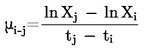(day–1)

where:

µ i-j:	is the average specific growth rate from time i to j;
X i :	is the biomass at time i;
X j :	is the biomass at time j.

For each treatment group and control group, calculate a mean value for growth rate along with variance estimates.

Calculate average specific growth rate over the entire test duration (normally days 0-3), using the nominally inoculated biomass as the starting value rather than a measured starting value, because in this way greater precision is normally obtained. If the equipment used for biomass measurement allows sufficiently precise determination of the low inoculum biomass (e.g. flow cytometer) then the measured initial biomass concentration can be used. Also assess the section-by-section growth rate, calculated as the specific growth rates for each day during the course of the test (days 0-1, 1-2 and 2-3) and examine whether the control growth rate remains constant (See validity criteria, section 1.7). A significantly lower specific growth rate on day one than the total average specific growth rate may indicate a lag phase. While a lag phase can be minimised and practically eliminated in control cultures by proper propagation of the pre-culture, a lag phase in exposed cultures may indicate recovery after initial toxic stress or reduced exposure due to loss of test substance (including sorption onto the algal biomass) after initial exposure. Hence the section-by-section growth rate may be assessed in order to evaluate effects of the test substance occurring during the exposure period. Substantial differences between the section-by-section growth rate and the average growth rate indicate deviation from constant exponential growth and that close examination of the growth curves is warranted.

Calculate the percent inhibition of growth rate for each treatment replicate from the equation:

where:

%Ir:	percent inhibition in average specific growth rate;
µC:	mean value for average specific growth rate (µ) in the control group;
µT:	average specific growth rate for the treatment replicate.

When solvents are used to prepare the test solutions, the solvent controls rather than the controls without solvents should be used in calculation of percent inhibition.

2.2.2.   Yield

The yield is calculated as the biomass at the end of the test minus the starting biomass for each single vessel of controls and treatments. For each test concentration and control, calculate a mean value for the yield along with variance estimates. The percentage inhibition in yield (%Iy) may be calculated for each treatment replicate as follows:

where:

%Iy:	percentage inhibition of yield;
YC:	mean value for yield in the control group;
YT:	value for yield for the treatment replicate.

2.3.   PLOTTING CONCENTRATION RESPONSE CURVE

Plot the percentage of inhibition against the logarithm of the test substance concentration and examine the plot closely, disregarding any such data point that was singled out as an outlier in the first phase. Fit a smooth line through the data points by eye or by computerised interpolation to get a first impression of the concentration response relationship, then proceed with a more detailed method, preferably a computerised statistical method. Depending on the intended usage of the data, the quality (precision) and amount of data, as well as the availability of data analysis tools, it may be decided (and sometimes well justified) to stop the data analysis at this stage and simply read the key figures EC50 and EC10 (and/or EC20) from the eye fitted curve (also see section below on stimulatory effects). Valid reasons for not using a statistical method may include:

—	data are not appropriate for computerised methods to produce any more reliable results than can be obtained by expert judgement — in such situations some computer programs may even fail to produce a reliable solution (iterations may not converge etc.),

—	stimulatory growth responses cannot be handled adequately using available computer programs (see below).

2.4.   STATISTICAL PROCEDURES

The aim is to obtain a quantitative concentration-response relationship by regression analysis. It is possible to use a weighted linear regression after having performed a linearising transformation of the response data — for instance into probit or logit or Weibull units (9), but non-linear regression procedures are preferred techniques that better handle unavoidable data irregularities and deviations from smooth distributions. Approaching either zero or total inhibition, such irregularities may be magnified by the transformation, interfering with the analysis (9). It should be noted that standard methods of analysis using probit, logit, or Weibull transforms are intended for use on quantal (e.g. mortality or survival) data, and must be modified to accommodate growth or biomass data. Specific procedures for determination of ECx values from continuous data can be found in (10)(11) and (12). The use of non-linear regression analysis is further detailed in Appendix 4.

For each response variable to be analysed, use the concentration-response relationship to calculate point estimates of ECx values. When possible, the 95 % confidence limits for each estimate should be determined. Goodness of fit of the response data to the regression model should be assessed either graphically or statistically. Regression analysis should be performed using individual replicate responses, not treatment group means. If, however, nonlinear curve fitting is difficult or fails because of too great a scatter in the data, the problem may be circumvented by performing the regression on group means as a practical way of reducing the influence of suspected outliers. Use of this option should be identified in the test report as a deviation from normal procedure because curve fits with individual replicates did not produce a good result.

EC50 estimates and confidence limits may also be obtained using linear interpolation with bootstrapping (13), if available regression models/methods are unsuitable for the data.

For estimation of the LOEC and hence the NOEC, and for effects of the test substance on growth rate, it is necessary to compare treatment means using analysis of variance (ANOVA) techniques. The mean for each concentration must then be compared with the control mean using an appropriate multiple comparison or trend test method. Dunnett’s or Williams’ test may be useful (14)(15)(16)(17)(18). It is necessary to assess whether the ANOVA assumption of homogeneity of variance holds. This assessment may be performed graphically or by a formal test (18). Suitable tests are Levene’s or Bartlett’s. Failure to meet the assumption of homogeneity of variances can sometimes be corrected by logarithmic transformation of the data. If heterogeneity of variance is extreme and cannot be corrected by transformation, analysis by methods such as step-down Jonkheere trend tests should be considered. Additional guidance on determining the NOEC can be found in (12).

Recent scientific developments have led to a recommendation of abandoning the concept of NOEC and replacing it with regression based point estimates ECx. An appropriate value for x has not been established for this algal test. A range of 10 to 20 % appears to be appropriate (depending on the response variable chosen), and preferably both the EC10 and EC20 should be reported.

2.5.   GROWTH STIMULATION

Growth stimulation (negative inhibition) at low concentrations is sometimes observed. This can result from either hormesis (toxic stimulation) or from addition of stimulating growth factors with the test material to the minimal medium used. Note that the addition of inorganic nutrients should not have any direct effect because the test medium should maintain a surplus of nutrients throughout the test. Low dose stimulation can usually be ignored in EC50 calculations unless it is extreme. However, if it is extreme, or an ECx value for low x is to be calculated, special procedures may be needed. Deletion of stimulatory responses from the data analysis should be avoided if possible, and if available curve fitting software cannot accept minor stimulation, linear interpolation with bootstrapping can be used. If stimulation is extreme, use of a hormesis model may be considered (19).

2.6.   NON-TOXIC GROWTH INHIBITION

Light absorbing test materials may give rise to a growth rate reduction because shading reduces the amount of available light. Such physical types of effects should be separated from toxic effects by modifying the test conditions and the former should be reported separately. Guidance may be found in (2) and (3).

3.   REPORTING

3.1.   TEST REPORT

The test report must include the following:

Test substance:

—	physical nature and relevant physiochemical properties, including water solubility limit,

—	chemical identification data, including purity.

Test species:

—	the strain, supplier or source and the culture conditions used.

Test conditions:

—	date of start of the test and its duration,

—	description of test design: test vessels, culture volumes, biomass density at the beginning of the test,

—	composition of the medium,

—	test concentrations and replicates (e.g. number of replicates, number of test concentrations and geometric progression used),

—	description of the preparation of test solutions, including use of solvents etc.,

—	culturing apparatus,

—	light intensity and quality (source, homogeneity),

—	temperature,

—	concentrations tested: the nominal test concentrations and any results of analyses to determine the concentration of the test substance in the test vessels. The recovery efficiency of the method and the limit of quantification in the test matrix should be reported,

—	all deviations from this Testing Method,

—	method for determination of biomass and evidence of correlation between the measured parameter and dry weight.

Results:

—	pH values at the start and end of the test at all treatments,

—	biomass for each flask at each measuring point and method for measuring biomass,

—	growth curves (plot of biomass versus time),

—	calculated response variables for each treatment replicate, with mean values and coefficient of variation for replicates,

—	graphical presentation of the concentration/effect relationship,

—	estimates of toxicity for response variables e.g. EC50, EC10, EC20 and associated confidence intervals. If calculated, LOEC and NOEC and the statistical methods used for their determination,

—	if ANOVA has been used, the size of the effect which can be detected (e.g. the least significant difference),

—	any stimulation of growth found in any treatment,

—	any other observed effects, e.g. morphological changes of the algae,

—	discussion of the results, including any influence on the outcome of the test resulting from deviations from this Testing Method.

4.   LITERATURE

(1)	OECD TG 201 (2006). Freshwater Alga and Cyanobacteria, Growth Inhibition Test.

(2)	ISO 1998: Water quality — Guidance for algal growth inhibition tests with poorly soluble materials, volatile compounds, metals and waster water. ISO/DIS 14442.

(3)	OECD 2000: Guidance Document on Aquatic Toxicity Testing of Difficult Substances and mixtures. Environmental Health and Safety Publications. Series on Testing and Assessment, no. 23.

(4)	ISO 1998: Water quality — Sampling — Part 16: General Guidance for Biotesting. ISO 5667-16.

(5)	ISO 1993: Water quality — Algal growth inhibition test. ISO 8692.

(6)	Mayer, P., Cuhel, R. and Nyholm, N. (1997). A simple in vitro fluorescence method for biomass measurements in algal growth inhibition tests. Water Research 31: 2525-2531.

(7)	Slovacey, R.E. and Hanna, P.J. In vivo fluorescence determinations of phytoplancton chlorophyll, Limnology & Oceanography 22,5 (1977), pp.919-925.

(8)	Simpson, S.L., Roland, M.G.E., Stauber, J.L. and Batley, G.E. (2003). Effect of declining toxicant concentrations on algal bioassay endpoints. Environ. Toxicol. Chem 22, 2073-2079.

(9)	Christensen, E.R., Nyholm, N. (1984): Ecotoxicological Assays with Algae: Weibull Dose-Response Curves. Env. Sci. Technol. 19, 713-718.

(10)	Nyholm, N. Sørensen, P.S., Kusk, K.O. and Christensen, E.R. (1992): Statistical treatment of data from microbial toxicity tests. Environ. Toxicol. Chem. 11, 157-167.

(11)	Bruce, R.D., and Versteeg, D.J. (1992). A statistical procedure for modelling continuous toxicity data. Env. Toxicol. Chem. 11:1485-1494.

(12)	OECD. (2004). Guidance Document on Statistical Analysis of Ecotoxicity Data.

(13)	Norberg-King T.J. (1988). An interpolation estimate for chronic toxicity: The ICp approach. National Effluent Toxicity Assessment Center Technical Report 05-88. USEPA, Duluth, MN.

(14)	Dunnett, C.W. (1955). A multiple comparisons procedure for comparing several treatments with a control. J. Amer. Statist. Assoc. 50: 1096-1121

(15)	Dunnett, C.W. (1964). New tables for multiple comparisons with a control. Biometrics 20: 482-491.

(16)	Williams, D.A. (1971). A test for differences between treatment means when several dose levels are compared with a zero dose control. Biometrics 27: 103-117.

(17)	Williams, D.A. (1972). The comparison of several dose levels with a zero dose control. Biometrics 28: 510-531.

(18)	Draper, N.R. and Smith, H. (1981). Applied Regression Analysis, second edition. Wiley, New York.

(19)	Brain P. and Cousens R. (1989). An equation to describe dose-responses where there is stimulation of growth at low doses. Weed Research, 29, 93-96.

ANNEX V

C.25.

AEROBIC MINERALISATION IN SURFACE WATER — SIMULATION BIODEGRADATION TEST

1.   METHOD

This method is equivalent to OECD TG 309 (2004) (1).

1.1.   INTRODUCTION

The purpose of this test is to measure the time course of biodegradation of a test substance at low concentration in aerobic natural water and to quantify the observations in the form of kinetic rate expressions. This simulation test is a laboratory shake flask batch test to determine rates of aerobic biodegradation of organic substances in samples of natural surface water (fresh, brackish or marine). It is based on the ISO/DIS 14592-1 (2) and it also includes elements from the testing methods C.23 and C.24 (3)(4). Optionally, with long test times, semi-continuous operation replaces batch operation in order to prevent deterioration of the test microcosm. The principal objective of the simulation test is to determine the mineralisation of the test substance in surface water, and mineralisation constitutes the basis for expressing degradation kinetics. However, an optional secondary objective of the test is to obtain information on the primary degradation and the formation of major transformation products. Identification of transformation products, and if possible quantification of their concentrations, are especially important for substances that are very slowly mineralised (e.g. with half-lives for total residual 14C exceeding 60 days). Higher concentrations of the test substance (e.g. > 100 μg/l) should normally be used for identification and quantification of major transformation products due to analytical limitations.

A low concentration in this test means a concentration (e.g. less than 1 μg/l to 100 μg/l) which is low enough to ensure that the biodegradation kinetics obtained in the test reflect those expected in the environment. Compared to the total mass of biodegradable carbon substrates available in the natural water used for the test, the test substance present at low concentration will serve as a secondary substrate. This implies that the anticipated biodegradation kinetics is first order (‘non-growth’ kinetics) and that the test substance may be degraded by ‘cometabolism’. First order kinetics implies that the rate of degradation (mg/L/day) is proportional to the concentration of substrate which declines over time. With true first order kinetics the specific degradation rate constant, k, is independent of time and concentration. That is, k does not vary appreciably during the course of an experiment and does not change with the added concentration between experiments. By definition, the specific degradation rate constant is equal to the relative change in concentration per time: k = (1/C) · (dC/dt). Although first order kinetics are normally expected under the prescribed conditions, there may be certain circumstances where other kinetics are more appropriate. Deviations from first order kinetics may e.g. be observed if mass transfer phenomena such as the diffusion rate, rather than the biological reaction rate, is limiting the rate of biotransformation. However, the data can nearly always be described by pseudo first order kinetics accepting a concentration dependent rate constant.

Information on biodegradability of the test substance at higher concentrations (e.g. from standard screening tests) as well as information on abiotic degradability, transformation products and relevant physico-chemical properties should be available prior to the test to help establish the experimental planning and interpret the results. The use of 14C labelled test substances and the determination of the phase distribution of 14C at the end of the test, enable ultimate biodegradability to be determined. When non-labelled test substance is used, ultimate biodegradation can only be estimated if a higher concentration is tested and all the major transformation products are known.

1.2.   DEFINITIONS

Primary biodegradation: The structural change (transformation) of a chemical substance by microorganisms resulting in the loss of chemical identity.

Functional biodegradation: The structural change (transformation) of a chemical substance by microorganisms resulting in the loss of a specific property.

Ultimate aerobic biodegradation: The breakdown of a chemical substance by microorganisms in the presence of oxygen to carbon dioxide, water and mineral salts of any other elements present (mineralisation) and the production of new biomass and organic microbial biosynthesis products.

Mineralisation: The breakdown of a chemical substance or organic matter by microorganisms in the presence of oxygen to carbon dioxide, water and mineral salts of any other elements present.

Lag phase: The time from the start of a test until adaptation of the degrading micro organisms is achieved and the biodegradation degree of a chemical substance or organic matter has increased to a detectable level (e.g. 10 % of the maximum theoretical biodegradation, or lower, dependent on the accuracy of the measuring technique).

Maximum level of biodegradation: The degree of biodegradation of a chemical substance or organic matter in a test, recorded in per cent, above which no further biodegradation takes place during the test.

Primary substrate: A collection of natural carbon and energy sources that provide growth and maintenance of the microbial biomass.

Secondary substrate: A substrate component present in such a low concentration, that by its degradation, only insignificant amounts of carbon and energy are supplied to the competent microorganisms, as compared to the carbon and energy supplied by the degradation of main substrate components (primary substrates).

Degradation rate constant: A first order or pseudo first order kinetic rate constant, k (d–1), which indicates the rate of degradation processes. For a batch experiment k is estimated from the initial part of the degradation curve obtained after the end of the lag phase.

Half-life, t1/2 (d): Term used to characterise the rate of a first order reaction. It is the time interval that corresponds to a concentration decrease by a factor 2. The half-life and the degradation rate constant are related by the equation t1/2 = ln2/k.

Degradation half time, DT50 (d): Term used to quantify the outcome of biodegradation tests. It is the time interval, including the lag phase, needed to reach a value of 50 % biodegradation.

Limit of detection (LOD) and limit of quantification (LOQ): The limit of detection (LOD) is the concentration of a substance below which the identity of the substance cannot be distinguished from analytical artefacts. The limit of quantification (LOQ) is the concentration of a substance below which the concentration cannot be determined with an acceptable accuracy.

Dissolved organic carbon (DOC): That part of the organic carbon in a sample of water which cannot be removed by specified phase separation, for example by centrifugation at 40 000 ms–2 for 15 min. or by membrane filtration using membranes with pores of 0,2 μm-0,45 μm diameter.

Total organic 14C activity (TOA): The total 14C activity associated with organic carbon.

Dissolved organic 14C activity (DOA): The total 14C activity associated with dissolved organic carbon.

Particulate organic 14C activity (POA): The total 14C activity associated with particulate organic carbon.

1.3.   APPLICABILITY OF THE TEST

This simulation test is applicable to non-volatile or slightly volatile organic substances tested at low concentrations. Using flasks open to the atmosphere (e.g. cotton wool plugged), substances with Henry’s law constants less than about 1 Pa·m3/mol (approx. 10–5 atm·m3/mol) can be regarded as non-volatile in practice. Using closed flasks with a headspace, it is possible to test slightly volatile substances (with Henry’s law constants < 100 Pa·m3/mol or < 10–3 atm·m3/mol) without losses from the test system. Loss of 14C-labelled substances may occur, if the right precautions are not exercised, when the CO2 is stripped off. In such situations, it may be necessary to trap CO2 in an internal absorber with alkali or to use an external CO2 absorber system (direct 14CO2 determination; see Appendix 3). For the determination of biodegradation kinetics, the concentrations of the test substance must be below its water solubility. It should be noted, however, that literature values of water solubility may be considerably higher than the solubility of the test substance in natural waters. Optionally, the solubility of especially poorly water-soluble test substances may be established by use of the natural waters being tested.

The method can be used for simulating biodegradation in surface water free of coarse particles (pelagic test) or in turbid surface water which, e.g. might exist near a water/sediment interface (suspended sediment test).

1.4.   PRINCIPLE OF THE TEST

The test is performed in batch by incubating the test substance with either surface water only (pelagic test) or surface water amended with suspended solids/sediment of 0,01 to 1 g/L dry weight (suspended sediment test) to simulate a water body with suspended solids or re-suspended sediment. The suspended solids/sediment concentration in the lower range of this interval is typical for most surface waters. The test flasks are incubated in darkness at an environmental temperature under aerobic conditions and agitation. At least two different concentrations of test substance should be used in order to determine the degradation kinetics. The concentrations should differ from each other by a factor of 5 to 10 and should represent the expected range of concentrations in the environment. The maximum concentration of the test substance should not exceed 100 µg/L, but maximum test concentrations below 10 µg/L or less are preferred to ensure that the biodegradation follows first order kinetics. The lowest concentration should not exceed 10 µg/L, but lowest test concentrations of 1-2 μg/L or less than 1 μg/L are preferred. Normally an adequate analysis of such low concentration can be achieved by use of commercially available 14C-labelled substances. Because of analytical limitations, it is frequently impossible to measure the concentration of the test substance with the required accuracy, if the test substance is applied at a concentration ≤ 100 µg/L (see second paragraph in section 1.7.2). Higher concentrations of test substance (> 100 µg/L and sometimes > 1 mg/L) may be used for the identification and quantification of major transformation products or if a specific analysis method with a low detection limit is not available. If high concentrations of test substance are tested, it may not be possible to use the results to estimate the first order degradation constant and half-life, as the degradation will probably not follow first order kinetics.

Degradation is followed at appropriate time intervals, by measuring either the residual 14C or the residual concentration of test substance when specific chemical analysis is used. 14C labelling of the most stable part of the molecule ensures the determination of the total mineralisation, while 14C labelling of a less stable part of the molecule, as well as the use of specific analysis, enable the assessment of only primary biodegradation. However, the most stable part does not necessarily include the relevant functional moiety of the molecule (that can be related to a specific property such as toxicity, bioaccumulation, etc.). If this is the case, it may be appropriate to use a test substance, which is 14C-labelled, in the functional part in order to follow the elimination of the specific property.

1.5.   INFORMATION ON THE TEST SUBSTANCE

Both radiolabelled and non-labelled test substances can be used in this test. 14C-labelling technique is recommended and labelling should normally be in the most stable part(s) of the molecule (see also section 1.4). For substances containing more than one aromatic ring, one or more carbons in each ring should preferably be 14C-labelled. In addition, one or more carbons on both sides of easily degradable linkages should preferably be 14C-labelled. The chemical and/or radiochemical purity of the test substance should be > 95 %. For radiolabelled substances, a specific activity of approx. 50 μCi/mg (1,85 MBq) or more is preferred in order to facilitate 14C measurements in tests conducted with low initial concentrations. The following information on the test substance should be available:

—	solubility in water [Method A.6],

—	solubility in organic solvent(s) (substances applied with solvent or with low solubility in water),

—	dissociation constant (pKa) if the substance is liable to protonation or deprotonation [OECD TG 112] (5),

—	vapour pressure [Method A.4] and Henry’s law constant,

—	chemical stability in water and in the dark (hydrolysis) [Method C.7].

When poorly water-soluble substances are being tested in seawater, it may also be useful to know the salting out constant (or ‘Setschenow constant’) Ks, which is defined by the expression: log (S/S’) = Ks Cm, where S and S’ are the solubility of the substance in fresh water and seawater, respectively, and Cm is the molar salt concentration.

If the test is carried out as a ‘suspended sediment test’ the following information should also be available:

—	n-octanol/water partition coefficient [Method A.8],

—	adsorption coefficient [Method C.18].

Other useful information may include:

—	environmental concentration, if known or estimated,

—	toxicity of the test substance to microorganisms [Method C.11],

—	ready and/or inherent biodegradability [Methods C.4 A-F, C.12, C.9, OECD TG 302 (5)],

—	aerobic or anaerobic biodegradability in soil and sediment/water transformation studies [Methods C.23, C.24].

1.6.   REFERENCE SUBSTANCE

A substance, which is normally easily degraded under aerobic conditions (e.g. aniline or sodium benzoate) should be used as reference substance. The expected time interval for degradation of aniline and sodium benzoate is usually less than 2 weeks. The purpose of the reference substances is to ensure that the microbial activity of the test water is within certain limits; i.e. that the water contains an active microbial population.

1.7.   QUALITY CRITERIA

1.7.1.   Recovery

Immediately after addition of the test substance, each initial test concentration should be verified by measurements of 14C activity, or by chemical analyses in the case of non-labelled substances, in at least duplicate samples. This provides information on the applicability and repeatability of the analytical method and on the homogeneity of the distribution of the test substance. Normally, the measured initial 14C activity or test substance concentration is used in the subsequent analyses of data rather than the nominal concentration as losses due to sorption and dosing errors thereby are compensated. For 14C-labelled test substance, the level of recovery at the end of the experiment is given by mass balance (see last paragraph in section 1.8.9.4). Ideally, the radiolabelled mass balance should range from 90 % to 110 %, whereas the analytical accuracy should lead to an initial recovery of between 70 % and 110 % for non-labelled test substances. These ranges should be interpreted as targets and should not be used as criteria for acceptance of the test. Optionally, the analytical accuracy may be determined for the test substance at a lower concentration than the initial concentration and for major transformation products.

1.7.2.   Repeatability and sensitivity of analytical method

Repeatability of the analytical method (including the efficiency of the initial extraction) to quantify the test substance, and transformation products, if appropriate, should be checked by five replicate analyses of the individual extracts of the surface water.

The limit of detection (LOD) of the analytical method for the test substance and for the transformation products should be at least 1 % of the initial amount applied to the test system if possible. The limit of quantification (LOQ) should be equal to or less than 10 % of the applied concentration. The chemical analyses of many organic substances and their transformation products frequently require that the test substance is applied at a relatively high concentration, i.e. > 100 μg/L.

1.8.   DESCRIPTION OF THE TEST METHOD

1.8.1.   Equipment

The test may be conducted in conical or cylindrical flasks of appropriate capacity (e.g. 0,5 or 1,0 litre) closed with silicone or rubber stoppers, or in serum flasks with CO2-tight lids (e.g. with butyl rubber septa). Another option is to perform the test by use of multiple flasks and to harvest whole flasks, at least in duplicate, at each sample interval (see last paragraph in section 1.8.9.1). For non-volatile test substances that are not radiolabelled, gas-tight stoppers or lids are not required; loose cotton plugs that prevent contamination from air are suitable (see second paragraph in section 1.8.9.1). Slightly volatile substances should be tested in a biometer-type system with gentle stirring of the water surface. To be sure that no bacterial contamination occurs, optionally the vessels can be sterilised by heating or autoclaving prior to use. In addition, the following standard laboratory equipment is used:

—	shaking table or magnetic stirrers for continuous agitation of the test flasks,

—	centrifuge,

—

pH meter,

—	turbidimeter for nephelometric turbidity measurements,

—	oven or microwave oven for dry weight determinations,

—	membrane filtration apparatus,

—	autoclave or oven for heat sterilisation of glassware,

—	facilities to handle 14C-labelled substances,

—	equipment to quantify 14C-activity in samples from CO2-trapping solutions and, if required, from sediment samples,

—	analytical equipment for the determination of the test (and reference) substance if specific chemical analysis is used (e.g. gas chromatograph, high-pressure liquid chromatograph).

1.8.2.   Stock solutions of test substance

Deionised water is used to prepare stock solutions of the test and reference substances (see first paragraph in section 1.8.7). The deionised water should be free of substances that may be toxic to microorganisms, and dissolved organic carbon (DOC) should be no more than 1 mg/L (6).

1.8.3.   Collection and transport of surface water

The sampling site for collection of the surface water should be selected in accordance with the purpose of the test in any given situation. In selecting sampling sites, the history of possible agricultural, industrial or domestic inputs must be considered. If it is known that an aquatic environment has been contaminated with the test substance or its structural analogues within the previous four years, it should not be used for the collection of test water, unless investigation of degradation rates in previously exposed sites is the express purpose of the investigator. The pH and temperature of the water should be measured at the site of collection. Furthermore, the depth of sampling and the appearance of the water sample (e.g. colour and turbidity) should be noted (see section 3). Oxygen concentration and/or redox potential in water and in the sediment surface layer should be measured in order to demonstrate aerobic conditions unless this is obvious as judged from appearance and historic experience with the site. The surface water should be transported in a thoroughly cleansed container. During transport, the temperature of the sample should not significantly exceed the temperature used in the test. Cooling to 4 °C is recommended if transport duration exceeds 2 to 3 hours. The water sample must not be frozen.

1.8.4.   Storage and preparation of surface water

The test should preferably be started within one day after sample collection. Storage of the water, if needed, should be minimised and must in any case not exceed a maximum of 4 weeks. The water sample should be kept at 4 °C with aeration until use. Prior to use, the coarse particles should be removed, e.g. by filtration through a nylon filter with about 100 μm mesh size or with a coarse paper filter, or by sedimentation.

1.8.5.   Preparation of water amended with sediment (optional)

For the suspended sediment test, surface sediment is added to the flasks containing natural water (filtered to remove coarse particles as described in section 1.8.4) to obtain a suspension; the concentration of suspended solids should be between 0,01 and 1 g/L. The surface sediment should come from the same site as that from which the water sample was taken. Dependent on the particular aquatic environment, the surface sediment may either be characterised by a high organic carbon content (2,5-7,5 %) and a fine texture or by a low organic carbon content (0,5-2,5 %) and a coarse texture (3). The surface sediment can be prepared as follows: extract several sediment cores using a tube of transparent plastic, slice off the upper aerobic layers (from surface to a depth of max. 5 mm) immediately after sampling and pool them together. The resulting sediment sample should be transported in a container with a large air headspace to keep the sediment under aerobic conditions (cool to 4 °C if transport duration exceeds 2-3 hours). The sediment sample should be suspended in the test water at a ratio of 1:10 and kept at 4 °C with aeration until use. Storage of the sediment, if needed, should be minimised and must not in any case exceed a maximum of 4 weeks.

1.8.6.   Semi-continuous procedure (optional)

Prolonged incubation (several months) may be necessary if a long lag time occurs before a significant degradation of the test substance can be measured. If this is known from previous testing of a substance, the test may be initiated by using a semi-continuous procedure, which allows periodical renewal of a part of the test water or suspension (see Appendix 2). Alternatively, the normal batch test may be changed into a semi-continuous test, if no degradation of the test substance has been achieved during approximately 60 days of testing using the batch procedure (see second paragraph in section 1.8.8.3).

1.8.7.   Addition of the test (or reference) substance

For substances with high water solubility (> 1 mg/L) and low volatility (Henry’s law constants < 1 Pa·m3/mol or < 10–5 atm·m3/mol), a stock solution can be prepared in deionised water (see section 1.8.2); the appropriate volume of the stock solution is added to the test vessels to achieve the desired concentration. The volume of any added stock solution should be held to the practical minimum (< 10 % of the final liquid volume, if possible). Another procedure is to dissolve the test substance in a larger volume of the test water, which may be seen as an alternative to the use of organic solvents.

If unavoidable, stock solutions of non-volatile substances with poor water-solubility should be prepared by use of a volatile organic solvent, but the amount of solvent added to the test system should not exceed 1 % v/v and should not have adverse effects on the microbial activity. The solvent should not affect the stability of the test substance in water. The solvent should be stripped off to an extremely small quantity so that it does not significantly increase the DOC concentration of the test water or suspension. This should be checked by substance-specific analysis or, if possible, DOC analysis (6). Care must be taken to limit the amount of solvent transferred to what is absolutely necessary, and to ensure that the amount of test substance can dissolve in the final volume of test water. Other techniques to introduce the test substance into the test vessels may be used as described in (7) and (8). When an organic solvent is used for application of the test substance, solvent controls containing the test water (with no additions) and test water with added reference substance should be treated similarly to active test vessels amended with test substance in solvent carrier. The purpose of the solvent controls is to examine possible adverse effects caused by the solvent towards the microbial population as indicated by the degradation of the reference substance.

1.8.8.   Test conditions

1.8.8.1.   Test temperature

Incubation should take place in the dark (preferred) or in diffuse light at a controlled (± 2 °C) temperature, which may be the field temperature or a standard temperature of 20-25 °C. Field temperature may be either the actual temperature of the sample at the sampling time or an average field temperature at the sampling site.

1.8.8.2.   Agitation

Agitation by means of continuous shaking or stirring must be provided to maintain particles and microorganisms in suspension. Agitation also facilitates oxygen transfer from the headspace to the liquid so that aerobic conditions can be adequately maintained. Place the flasks on a shaking table (approx. 100 rpm agitation) or use magnetic stirring. Agitation must be continuous. However, the shaking or stirring should be as gentle as possible, while still maintaining a homogeneous suspension.

1.8.8.3.   Test duration

The duration of the test should normally not exceed 60 days unless the semi-continuous procedure with periodical renewal of the test suspension is applied (see section 1.8.6 and Appendix 2). However, the test period for the batch test may be extended to a maximum of 90 days, if the degradation of the test substance has started within the first 60 days. Degradation is monitored, at appropriate time intervals, by the determination of the residual 14C activity or the evolved 14CO2 (see section 1.8.9.4) and/or by chemical analysis (section 1.8.9.5). The incubation time must be sufficiently long to evaluate the degradation process. The extent of degradation should preferably exceed 50 %; for slowly degradable substances, the extent of degradation must be sufficient (normally greater than 20 % degradation) to ensure the estimation of a kinetic degradation rate constant.

Periodic measurements of pH and oxygen concentration in the test system must be conducted unless previous experience from similar tests with water and sediment samples collected from the same site make such measurements unnecessary. Under some conditions, the metabolism of primary substrates at much higher concentrations within the water or sediment could possibly result in enough CO2 evolution and oxygen depletion to significantly alter the experimental conditions during the test.

1.8.9.   Procedure

1.8.9.1.   Preparation of flasks for pelagic test

Transfer a suitable volume of test water to the test flasks, up to about one third of the flask volume and not less than about 100 ml. If multiple flasks are used (to allow harvesting of whole flasks at each sampling time), the appropriate volume of test water is also about 100 ml, as small sample volumes may influence the length of the lag phase. The test substance is added from a stock solution as described in sections 1.8.2 and 1.8.7. At least two different concentrations of test substance differing by a factor of 5 to 10 should be used in order to determine degradation kinetics and calculate the kinetic degradation rate constant. Both of the selected concentrations should be less than 100 µg/L and preferably in the range of < 1-10 µg/L.

Close the flasks with stoppers or lids impermeable to air and CO2. For non-14C-labelled non-volatile test chemicals, loose cotton wool plugs that prevent contamination from air are suitable (see section 1.8.1) provided that any major degradation products are known to be non-volatile, and if indirect CO2 determination is used (see Appendix 3).

Incubate the flasks at the selected temperature (see section 1.8.8.1). Withdraw samples for chemical analysis or 14C measurements at the beginning of the test (i.e. before biodegradation starts; see section 1.7.1) and then at suitable time intervals during the course of the test. Sampling may be performed by withdrawal of sub-samples (e.g. 5 ml aliquots) from each replicate or by harvest of whole flasks at each sampling time. The mineralisation of the test substance may either be determined indirectly or directly (see Appendix 3). Usually, a minimum of five sampling points are required during the degradation phase (i.e. after ended lag phase) in order to estimate a reliable rate constant, unless it can be justified that three sampling points are sufficient for rapidly degradable substances. For substances that are not rapidly degraded more measurements during the degradation phase can easily be made and, therefore, more data points should be used for the estimation of k. No fixed time schedule for sampling can be stated, as the rate of biodegradation varies; however the recommendation is to sample once a week if degradation is slow. If the test substance is rapidly degradable, sampling should take place once a day during the first three days and then every second or third day. Under certain circumstances, such as with very rapidly hydrolysing substances, it may be necessary to sample at hourly intervals. It is recommended that a preliminary study is conducted prior to the test in order to determine the appropriate sampling intervals. If samples have to be available for further specific analysis, it is advisable to take more samples and then select those to be analysed at the end of the experiment following a backwards strategy, i.e. the last samples are analysed first (see second paragraph in section 1.8.9.5 for guidance on stability of samples during storage).

1.8.9.2.   Number of flasks and samples

Set up a sufficient number of test flasks to have:

—	test flasks; at least duplicate flasks for each concentration of test substance (preferably a minimum of 3) or multiple test flasks for each concentration, if whole flasks are harvested at each sampling time (symbolised FT),

—	test flasks for mass balance calculation; at least duplicate flasks for each test concentration (symbolised FM),

—	blank control, no test substance; at least one blank test flask containing only the test water (symbolised FB),

—

reference control; duplicate flasks with reference substance (e.g. aniline or sodium benzoate, at 10 µg/l) (symbolised FC). The purpose of the reference control is to confirm a minimum of microbial activity. If convenient, a radiolabelled reference substance may be used, also when the degradation of the test substance is monitored by chemical analyses,

—

sterile control; one or two flasks containing sterilised test water for examining possible abiotic degradation or other non-biological removal of the test substance (symbolised FS). The biological activity can be stopped by autoclaving (121 °C; 20 min.) the test water or by adding a toxicant (e.g. sodium azide (NaN3) at 10-20 g/l, mercuric chloride (HgCl2) at 100 mg/l or formalin at 100 mg/l) or by gamma irradiation. If HgCl2 is used, it should be disposed of as toxic waste. For water with sediment added in large amount, sterile conditions are not easy to obtain; in this case repeated autoclaving (e.g. three times) is recommended. It should be considered that the sorption characteristics of the sediment may be altered by autoclaving,

—

solvent controls, containing test water and test water with reference substance; duplicate flasks treated with the same amount of solvent and by use of the same procedure as that used for application of the test substance. The purpose is to examine possible adverse effects of the solvent by determining the degradation of the reference substance.

In the design of the test, the investigator should consider the relative importance of increased experimental replication versus increased number of sampling times. The exact number of flasks required will depend on the method used for measuring the degradation (see third paragraph in section 1.8.9.1; section 1.8.9.4 and Appendix 3).

Two subsamples (e.g. 5 ml aliquots) should be withdrawn from each test flask at each sampling time. If multiple flasks are used to allow harvesting of whole flasks, a minimum of two flasks should be sacrificed at each sampling time (see first paragraph in section 1.8.9.1).

1.8.9.3.   Preparation of flasks for suspended sediment test [optional]

Add the necessary volumes of test water and sediment, if required, to the test vessels (see section 1.8.5). The preparation of flasks for suspended sediment test is the same as for the pelagic test (see sections 1.8.9.1 and 1.8.9.2). Use preferably serum bottles or similar shaped flasks. Place the closed flasks horizontally on a shaker. Obviously, open flasks for non-14C-labelled, non-volatile substances should be placed in upright position; in this case magnetic stirring and the use of magnetic bars coated with glass are recommended. If necessary, aerate the bottles to maintain proper aerobic conditions.

1.8.9.4.   Radiochemical determinations

The evolved 14CO2 is measured indirectly and directly (see Appendix 3). The 14CO2 is determined indirectly by the difference between the initial 14C activity in the test water or suspension and the total residual activity at the sampling time as measured after acidifying the sample to pH 2-3 and stripping off CO2. Inorganic carbon is thus removed and the residual activity measured derives from organic material. The indirect 14CO2 determination should not be used, if major volatile transformation products are formed during the transformation of the test substance (see Appendix 3). If possible, the 14CO2 evolution should be measured directly (see Appendix 3) at each sampling time in at least one test flask; this procedure enables both the mass balance and biodegradation process to be checked, but it is restricted to tests conducted with closed flasks.

If the evolved 14CO2 is measured directly during the test, more flasks should be set up for this purpose at the start of the test. Direct 14CO2 determination is recommended, if major volatile transformation products are formed during the transformation of the test substance. At each measuring point the additional test flasks are acidified to pH 2-3 and the 14CO2 is collected in an internal or external absorber (see Appendix 3).

Optionally the concentrations of 14C-labelled test substance and major transformation products may be determined by use of radiochromatography (e.g. thin layer chromatography, RAD-TLC) or HPLC with radiochemical detection.

Optionally the phase distribution of the remaining radioactivity (see Appendix 1) and residual test substance and transformation products may be determined.

At the end of the test the mass balance should be determined by direct 14CO2 measurement using separate test flasks from which no samples are taken in the course of the test (see Appendix 3).

1.8.9.5.   Specific chemical analysis

If a sensitive specific analytical method is available, primary biodegradation can be assessed by measuring the total residual concentration of test substance instead of using radiolabelling techniques. If a radiolabelled test substance is used (to measure total mineralisation), specific chemical analyses can be made in parallel to provide useful additional information and check the procedure. Specific chemical analyses may also be used to measure transformation products formed during the degradation of the test substance, and this is recommended for substances that are mineralised with half-lives exceeding 60 days. The concentration of the test substance and the transformation products at every sampling time should be measured and reported (as a concentration and as percentage of applied). In general, transformation products detected at ≥ 10 % of the applied concentration at any sampling time should be identified unless reasonably justified otherwise. Transformation products for which concentrations are continuously increasing during the study should also be considered for identification, even if their concentrations do not exceed the limit given above, as this may indicate persistence. Analyses of transformation products in sterile controls should be considered, if rapid abiotic transformation of the test substance (e.g. hydrolysis) is thought possible. The need for quantification and identification of transformation products should be considered on a case by case basis, with justifications being provided in the report. Extraction techniques with organic solvent should be applied according to directions given in the respective analytical procedure.

All samples should be stored at 2 to 4 °C and air-tight if analysis is carried out within 24 hours (preferred). For longer storage, the samples should be frozen below –  18 °C or chemically preserved. Acidification is not a recommended method to preserve the samples, because acidified samples may be unstable. If the samples are not analysed within 24 hours and are subject to longer storage, a storage stability study should be conducted to demonstrate the stability of chemicals of interest under –  18 °C storage or preserved conditions. If the analytical method involves either solvent extraction or solid phase extraction (SPE), the extraction should be performed immediately after sampling or after storing the sample refrigerated for a maximum of 24 hours.

Depending on the sensitivity of the analytical method, larger sample volumes than those indicated in section 1.8.1 may be necessary. The test can easily be carried out with test volumes of one litre in flasks of 2-3 litre volume, which makes it possible to collect samples of approx. 100 ml.

2.   DATA AND REPORTING

2.1.   TREATMENT OF RESULTS

2.1.1.   Plot of data

Round off sampling times to a whole number of hours (unless the substance degrades substantially in a matter of minutes to hours) but not to a whole number of days. Plot the estimates of the residual activity of test substance (for 14C-labelled substances) or the residual concentration (for non-labelled substances), against time both in a linear and in a semi-logarithmic plot (see Figures 1a, 1b). If degradation has taken place, compare the results from flasks FT with those from flasks FS. If the means of the results from the flasks with test substance (FT) and the sterile flasks (FS) deviate by less than 10 %, it can be assumed that the degradation observed is predominantly abiotic. If the degradation in flasks FS is lower, the figures may be used to correct those obtained with flasks FT (by subtraction) in order to estimate the extent of biodegradation. When optional analyses are performed for major transformation products, plots of their formation and decline should be provided in addition to a plot of the decline of the test substance.

Estimate the lag phase duration tL from the degradation curve (semi-logarithmic plot) by extrapolating its linear part to zero degradation or alternatively by determining the time for approximately 10 % degradation (see Figures 1a and 1b). From the semi-logarithmic plot, estimate the first order rate constant, k, and its standard error by linear regression of ln (residual 14C activity or test substance concentration) versus time. With 14C measurements in particular, use only data belonging to the initial linear part of the curve after the ended lag phase, and give preference to selecting few and representative data rather than selecting a greater number of more uncertain data. Uncertainty includes here errors inherent in the recommended direct use of measured residual 14C activities (see below). It may sometimes be relevant to calculate two different rate constants, if the degradation follows a biphasic pattern. For this purpose two different phases of the degradation curve are defined. Calculations of the rate constant, k, and the half-life t½ = ln2/k, should be carried out for each of the individual replicate flasks, when sub-samples are withdrawn from the same flask, or by using the average values, when whole flasks are harvested at each sampling time (see last paragraph in section 1.8.9.2). When the first-mentioned procedure is used, the rate constant and half-life should be reported for each of the individual replicate flasks and as an average value with a standard error. If high concentrations of test substance have been used, the degradation curve may deviate considerably from a straight line (semi-logarithmic plot) and first order kinetics may not be valid. Defining a half-life has therefore no meaning. However, for a limited data range, pseudo first order kinetics can be applied and the degradation half-time DT50 (time to reach 50 % degradation) estimated. It must be borne in mind, however, that the time course of degradation beyond the selected data range cannot be predicted using the DT50 which is merely a descriptor of a given set of data. Analytical tools to facilitate statistical calculations and curve fitting are easily available and the use of this kind of software is recommended.

If specific chemical analyses are made, estimate rate constants and half-lives for primary degradation as above for total mineralisation. If the primary degradation is the limiting process data points from the entire course of degradation may sometimes be used. This is because measurements are direct by contrast to measurements of 14C activity.

If 14C-labelled substances are used, a mass balance should be expressed in percentage of the applied initial concentration, at least at the end of the test.

2.1.2.   Residual activity

When the 14C-labelled part of an organic substance is biodegraded, the major part of the 14C is converted to 14CO2, while another part is used for growth of biomass and/or synthesis of extra-cellular metabolites. Therefore, complete ‘ultimate’ biodegradation of a substance does not result in a 100 % conversion of its carbon into 14CO2. The 14C built into products formed by biosynthesis is subsequently released slowly as 14CO2 due to ‘secondary mineralisation’. For these reasons plots of residual organic 14C activity (measured after stripping off CO2) or of 14CO2 produced versus time will show a ‘tailing’ after degradation has been completed. This complicates a kinetic interpretation of the data and for this purpose, only the initial part of the curve (after the lag phase has ended and before approx. 50 % degradation is reached) should normally be used for the estimation of a degradation rate constant. If the test substance is degraded, the total residual organic 14C activity is always higher than the 14C activity associated with the remaining intact test substance. If the test substance is degraded by a first order reaction and a constant fraction α is mineralised into CO2, the initial slope of the 14C disappearance curve (total organic 14C versus time) will be α times the slope of the corresponding curve for the concentration of test substance (or, to be precise, the part of the test substance labelled with 14C). Using measurements of the total organic 14C activity uncorrected, the calculated degradation rate constant will therefore be conservative. Procedures for estimating the concentrations of the test substance from the measured radiochemical activities based on various simplifying assumptions have been described in the literature (2)(9)(10)(11). Such procedures are most easily applied for rapidly degradable substances.

2.2.   INTERPRETATION OF RESULTS

If k is found to be independent of the added concentration (i.e. if the calculated k is approximately the same at the different concentrations of test substance), it can be assumed that the first order rate constant is representative of the testing conditions used, i.e. the test substance, the water sample and the test temperature. To what extent the results can be generalised or extrapolated to other systems must be evaluated by expert judgement. If a high concentration of test substance is used, and the degradation therefore does not follow first order kinetics, the data cannot be used for direct estimation of a first order rate constant or a corresponding half-life. However, data derived from a test using a high concentration of test substance may still be usable for estimating the degree of total mineralisation and/or detection and quantification of transformation products.

If the rates of other loss processes than biodegradation are known (e.g. hydrolysis or volatilisation), they may be subtracted from the net loss rate observed during the test to give an approximated estimate of the biodegradation rate. Data for hydrolysis may, e.g. be obtained from the sterile control or from parallel testing using a higher concentration of the test substance.

The indirect and direct determination of 14CO2 (section 1.8.9.4 and Appendix 3) can only be used to measure the extent of mineralisation of the test substance to CO2. Radiochromatography (RAD-TLC) or HPLC may be used to analyse the concentrations of 14C-labelled test substance and the formation of major transformation products (third paragraph in section 1.8.9.4). To enable a direct estimation of the half-life, it is necessary that no major transformation products (defined as ≥ 10 % of the applied amount of test substance) be present. If major transformation products as defined here are present, a detailed evaluation of the data is required. This may include repeated testing and/or identification of the transformation products (see first paragraph in section 1.8.9.5) unless the fate of the transformation products can be reasonably assessed by use of experience (e.g. information on degradation pathway). As the proportion of test substance carbon converted to CO2 varies (depending largely on the concentration of test substance and other substrates available, the test conditions and the microbial community), this test does not allow a straightforward estimation of ultimate biodegradation as in a DOC die-away test; but the result is similar to that obtained with a respirometric test. The degree of mineralisation will thus be less than or equal to the minimum level of ultimate biodegradation. To obtain a more complete picture of the ultimate biodegradation (mineralisation and incorporation into biomass), the analysis of the phase distribution of 14C should be performed at the end of the test (see Appendix 1). The 14C in the particulate pool will consist of 14C incorporated into bacterial biomass and 14C sorbed to organic particles.

2.3.   VALIDITY OF THE TEST

If the reference substance is not degraded within the expected time interval (for aniline and sodium benzoate, usually less than two weeks), the validity of the test is suspected and must be further verified, or alternatively the test should be repeated with a new water sample. In an ISO ring-test of the method where seven laboratories located around Europe participated, adapted degradation rate constants for aniline ranged from 0,3 to 1,7 day–1 with an average of 0,8 d–1 at 20 oC and a standard error of ±0,4 d–1 (t½ = 0,9 days). Typical lag times were 1 to 7 days. The waters examined were reported to have a bacterial biomass corresponding to 103 -104 colony forming units (CFU) per ml. Degradation rates in nutrient-rich Mid-European waters were greater than in Nordic oligotrophic waters, which may be due to the different trophic status or previous exposure to chemical substances.

The total recovery (mass balance) at the end of the experiment should be between 90 % and 110 % for radiolabelled substances, whereas the initial recovery at the beginning of the experiment should be between 70 % and 110 % for non-labelled substances. However, the indicated ranges should only be interpreted as targets and should not be used as criteria for acceptance of the test.

3.   TEST REPORT

The type of study, i.e. pelagic or suspended sediment test, must be clearly stated in the test report, which shall also contain at least the following information:

Test substance and reference substance(s):

—	common names, chemical names (recommend IUPAC and/or CAS names), CAS numbers, structural formulas (indicating position of 14C if radiolabelled substance is used) and relevant physico-chemical properties of test and reference substance (see sections 1.5 and 1.6),

—	chemical names, CAS numbers, structural formulas (indicating position of 14C if radiolabelled substance is used) and relevant physico-chemical properties of substances used as standards for identification and quantification of transformation products,

—	purity (impurities) of test and reference substances,

—	radiochemical purity of labelled chemical and specific activity (where appropriate).

Surface water:

The following minimum information for the water sample taken must be provided:

—	location and description of sampling site including, if possible, contamination history,

—	date and time of sample collection,

—	nutrients (total N, ammonium, nitrite, nitrate, total P, dissolved orthophosphate),

—	depth of collection,

—	appearance of sample (e.g. colour and turbidity),

—	DOC and TOC,

—

BOD,

—	temperature and pH at the place and time of collection,

—	oxygen or redox potential (mandatory only if aerobic conditions are not obvious),

—	salinity or conductivity (in the case of sea water and brackish water),

—	suspended solids (in case of a turbid sample),

—	possibly other relevant information about the sampling location at the time of sampling (e.g. actual or historical data on flow rate of rivers or marine currents, nearby major discharges and type of discharges, weather conditions preceding the sampling time),

and optionally:

—	microbial biomass (e.g. acridine orange direct count or colony forming units),

—	inorganic carbon,

—	chlorophyll-a concentration as a specific estimate for algal biomass.

In addition, the following information on the sediment should be provided if the suspended sediment test is conducted:

—	depth of sediment collection,

—	appearance of the sediment (such as coloured, muddy, silty, or sandy),

—	texture (e.g. % coarse sand, fine sand, silt and clay),

—	dry weight in g/l of the suspended solids, TOC concentration or weight loss on ignition as a measure of the content of organic matter,

—

pH,

—	oxygen or redox potential (mandatory only if aerobic conditions are not obvious).

Test conditions:

—	delay between collection and use in the laboratory test, sample storage and pre-treatment of the sample, dates of performance of the studies,

—	amount of test substance applied, test concentration and reference substance,

—	method of application of the test substance including any use of solvents,

—	volume of surface water used and sediment (if used) and volume sampled at each interval for analysis,

—	description of the test system used.

If dark conditions are not to be maintained, information on the ‘diffuse light’ conditions:

—	information on the method(s) used for establishing sterile controls (e.g. temperature, time and number of autoclavings),

—	incubation temperature,

—	information on analytical techniques and the method(s) used for radiochemical measurements and for mass balance check and measurements of phase distribution (if conducted),

—	number of replicates.

Results:

—	percentages of recovery (see section 1.7.1),

—	repeatability and sensitivity of the analytical methods used including the limit of detection (LOD) and the limit of quantification (LOQ) (see section 1.7.2),

—

all measured data (including sampling time points) and calculated values in tabular form and the degradation curves; for each test concentration and for each replicate flask, report the linear correlation coefficient for the slope of the logarithmic plot, the estimated lag phase and a first-order or pseudo-first order rate constant (if possible), and the corresponding degradation half-life (or the half-life period, t50),

—	report relevant values as the averages of the results observed in individual replicates, e.g. length of lag phase, degradation rate constant and degradation half-life (or t50),

—	categorise the system as either non-adapted or adapted as judged from the appearance of the degradation curve and from the possible influence of the test concentration,

—	the results of the final mass balance check and results on phase distribution measurements (if any),

—	the fraction of 14C mineralised and, if specific analyses are used, the final level of primary degradation,

—	the identification, molar concentration and percentage of applied and major transformation products (see first paragraph in section 1.8.9.5), where appropriate,

—	a proposed pathway of transformation, where appropriate,

—	discussion of results.

4.   LITERATURE

1.	OECD TG 309 (2004) Aerobic Mineralisation in surface water — Simulation Biodegradation Test.

2.	ISO/DIS 14592-1 (1999) Water quality — Evaluation of the aerobic biodegradability of organic compounds at low concentrations — Part 1: Shake flask batch test with surface water or surface water/sediment suspensions.

3.	Testing Method C.23. Aerobic and anaerobic transformation in soil.

4.	Testing Method C.24. Aerobic and anaerobic transformation in aquatic sediments.

5.	OECD (1993). Guidelines for the Testing of Chemicals. OECD, Paris.

6.	ISO 8245 (1999). Water quality — Guidelines on the determination of total organic carbon (TOC) and dissolved organic carbon (DOC).

7.	ISO 10634 (1995). Water quality — Guidance for the preparation and treatment of poorly water-soluble organic compounds for the subsequent evaluation of their biodegradability in an aqueous medium.

8.	OECD (2000). Guidance Document on aquatic toxicity testing of difficult substances and mixtures. Environmental Health and Safety Publications. Series on Testing and Assessment. No 22.

9.	Simkins, S. and Alexander, M. (1984). Models for mineralisation kinetics with the variables of substrate concentration and population density. Appl. Environ. Microbiol.47, 394-401.

10.	Ingerslev, F. and N. Nyholm. (2000). Shake-flask test for determination of biodegradation rates of 14C-labeled chemicals at low concentrations in surface water systems. Ecotoxicol. Environ. Saf. 45, 274-283.

11.	ISO/CD 14592-1 (1999). Ring test report: Water Quality — Evaluation of the aerobic biodegradability of organic compounds at low concentrations part 1 — report of 1998/1999 ring-test. Shake flask batch test with surface water or surface water/sediment suspensions.

ANNEX VI

C.26.

LEMNA SP. GROWTH INHIBITION TEST

1.   METHOD

This method is equivalent to OECD TG 221 (2006) (1). There has been broad agreement by EU authorities that the Lemna test is a suitable alternative to an algal test for strongly coloured substances (2)(3).

1.1.   INTRODUCTION

This Testing Method is designed to assess the toxicity of substances to freshwater aquatic plants of the genus Lemna (duckweed). It is based on existing guidelines (4)(5)(6)(7)(8)(9) but includes modifications of those methods to reflect recent research and consultation on a number of key issues. The proposed method has been validated by an international ring-test (10).

This Testing Method describes toxicity testing using Lemna gibba and Lemna minor, both of which have been extensively studied and are the subject of the standards referred to above. The taxonomy of Lemna spp. is difficult, being complicated by the existence of a wide range of phenotypes. Although genetic variability in the response to toxicants can occur with Lemna, there are currently insufficient data on this source of variability to recommend a specific clone for use with this Testing Method. It should be noted that the test is not conducted axenically, but steps are taken at stages during the test procedure to keep contamination by other organisms to a minimum.

Details on testing with renewal (semi-static and flow-through) and without renewal (static) of the test solution are described. Depending on the objectives of the test and on the regulatory requirements, it is recommended to consider the application of semi-static and flow through methods, e.g. for substances that are rapidly lost from solution as a result of volatilisation, photodegradation, precipitation or biodegradation. Further guidance is given in (11).

1.2.   DEFINITIONS

The following definitions and abbreviations are used for the purposes of this Testing Method:

Biomass: is the dry weight of living matter present in a population. In this test, surrogates for biomass, such as frond counts or frond area, are typically measured and the use of the term ‘biomass’ thus refers to these surrogate measures as well.

Chlorosis: is the yellowing of frond tissue.

Clone: is an organism or cell arisen from a single individual by asexual reproduction. Individuals from the same clone are, therefore, genetically identical.

Colony: means an aggregate of mother and daughter fronds (usually 2 to 4) attached to each other. Sometimes referred to as a plant.

ECx : is the concentration of the test substance dissolved in test medium that results in an x % (e.g. 50 %) reduction in growth of Lemna within a stated exposure period (to be mentioned explicitly if deviating from full or normal test duration). To unambiguously denote an EC value deriving from growth rate or yield, the symbol ‘ErC’ is used for growth rate and ‘EyC’ is used for yield, followed by the measurement variable used, e.g. ErC (frond number).

Flow-through: is a test in which the test solutions are replaced continuously.

Frond: is an individual/single ‘leaf-like’ structure of a duckweed plant. It is the smallest unit, i.e. individual, capable of reproduction.

Gibbosity: means fronds exhibiting a humped or swollen appearance.

Growth: is an increase in the measurement variable, e.g. frond number, dry weight, wet weight or frond area, over the test period.

Growth rate (average specific growth rate): is the logarithmic increase in biomass during the exposure period.

Lowest Observed Effect Concentration (LOEC): is the lowest tested concentration at which the substance is observed to have a statistically significant reducing effect on growth (at p < 0,05) when compared with the control, within a given exposure time. However, all test concentrations above the LOEC must have a harmful effect equal to or greater than those observed at the LOEC. When these two conditions cannot be satisfied, a full explanation must be given for how the LOEC (and hence the NOEC) has been selected.

Measurement variables: are any type of variables which are measured to express the test endpoint using one ore more different response variables. In this method frond number, frond area, fresh weight and dry weight are measurement variables.

Monoculture: is a culture with one plant species.

Necrosis: is dead (i.e. white or water-soaked) frond tissue.

No Observed Effect Concentration (NOEC): is the test concentration immediately below the LOEC.

Phenotype: is the observable characteristics of an organism determined by the interaction of its genes with its environment.

Response variables: are variables for the estimation of toxicity derived from any measured variables describing biomass by different methods of calculation. For this method, growth rates and yield are response variables derived from measurement variables like frond number, frond area, fresh weight or dry weight.

Semi-static (renewal) test: is a test in which the test solution is periodically replaced at specific intervals during the test.

Static test: is a test method without renewal of the test solution during the test.

Test endpoint: describes the general factor that will be changed by the test chemical relative to the control as aim of the test. In this method the test endpoint is inhibition of growth, which may be expressed by different response variables which are based on one or more measurement variables.

Test medium: is the complete synthetic growth medium on which test plants grow when exposed to the test substance. The test substance will normally be dissolved in the test medium.

Yield: is the value of a measurement variable to express biomass at the end of the exposure period minus the measurement variable at the start of the exposure period.

1.3.   PRINCIPLE OF THE TEST

Exponentially growing plant cultures of the genus Lemna are allowed to grow as monocultures in different concentrations of the test substance over a period of seven days. The objective of the test is to quantify substance-related effects on vegetative growth over this period, based on assessments of selected measurement variables. Frond number is the primary measurement variable. At least one other measurement variable (total frond area, dry weight or fresh weight) is also measured, since some substances may affect other measurement variables much more than frond numbers. To quantify substance-related effects, growth in the test solutions is compared with that of the controls and the concentration bringing about a specified x % inhibition of growth (e.g. 50 %) is determined and expressed as the ECx (e.g. EC50).

The test endpoint is inhibition of growth, expressed as logarithmic increase in the measurement variable (average specific growth rate) during the exposure period. From the average specific growth rates recorded in a series of test solutions, the concentration bringing about a specified x % inhibition of growth rate (e.g. 50 %) is determined and expressed as the ErCx (e.g. ErC50).

An additional response variable used in this Testing Method is yield, which may be needed to fulfil specific regulatory requirements in some countries. It is defined as the measurement variables at the end of the exposure period minus the measurement variables at the start of the exposure period. From the yield recorded in a series of test solutions, the concentration bringing about a specified x % inhibition of yield (e.g. 50 %) is calculated and expressed as the EyCx (e.g. EyC50).

In addition, the lowest observed effect concentration (LOEC) and the no observed effect concentration (NOEC) may be statistically determined.

1.4.   INFORMATION ON THE TEST SUBSTANCE

An analytical method, with adequate sensitivity for quantification of the substance in the test medium, should be available.

Information on the test substance which may be useful in establishing the test conditions includes the structural formula, purity, water solubility, stability in water and light, pKa, Kow, vapour pressure and biodegradability. Water solubility and vapour pressure can be used to calculate Henry’s Law constant, which will indicate if significant losses of the test substance during the test period are likely. This will help indicate whether particular steps to control such losses should be taken. Where information on the solubility and stability of the test substance is uncertain, it is recommended that these be assessed under the conditions of the test, i.e. growth medium, temperature, lighting regime to be used in the test.

When pH control of the test medium is particularly important, e.g. when testing metals or substances which are hydrolytically unstable, the addition of a buffer to the growth medium is recommended (see first paragraph in section 1.7.4). Further guidance for testing substances with physicochemical properties that make them difficult to test is provided in (11).

1.5.   REFERENCE SUBSTANCE

Reference substance(s), such as 3,5-dichlorophenol used in the international ring test (10), may be tested as a means of checking the test procedure. It is advisable to test a reference substance at least twice a year or, where testing is carried out at a lower frequency, in parallel to the determination of the toxicity of a test substance.

1.6.   VALIDITY OF THE TEST

For the test to be valid, the doubling time of frond number in the control must be less than 2,5 days (60 h), corresponding to approximately a seven-fold increase in seven days and an average specific growth rate of 0,275 d–1. Using the media and test conditions described in this Testing Method, this criterion can be attained using a static test regime (8). It is also anticipated that this criterion will be achievable under semi-static and flow-through test conditions. Calculation of the doubling time is shown in section 2.1.

1.7.   DESCRIPTION OF THE METHOD

1.7.1.   Apparatus

All equipment in contact with the test media should be made of glass or other chemically inert material. Glassware used for culturing and testing purposes should be cleaned of chemical contaminants that might leach into the test medium and should be sterile. The test vessels should be wide enough for the fronds of different colonies in the control vessels to grow without overlapping at the end of the test. It does not matter if the roots touch the bottoms of the test vessels, but a minimum depth of 20 mm and minimum volume of 100 ml in each test vessel is advised. The choice of test vessels is not critical as long as these requirements are met. Glass beakers, crystallising dishes or glass petri dishes of appropriate dimensions have all proved suitable. Test vessels must be covered to minimise evaporation and accidental contamination, while allowing necessary air exchange. Suitable test vessels, and particularly covers, must avoid shadowing or changes in the spectral characteristics of light.

The cultures and test vessels should not be kept together. This is best achieved using separate environmental growth chambers, incubators, or rooms. Illumination and temperature must be controllable and maintained at a constant level (see section 1.7.8).

1.7.2.   Test organism

The organism used for this test is either Lemna gibba or Lemna minor. Short descriptions of duckweed species that have been used for toxicity testing are given in Appendix 1. Plant material may be obtained from a culture collection, another laboratory or from the field. If collected from the field, plants should be maintained in culture in the same medium as used for testing for a minimum of eight weeks prior to use. Field sites used for collecting starting cultures must be free of obvious sources of contamination. If obtained from another laboratory or from a culture collection they should be similarly maintained for a minimum of three weeks. The source of plant material and the species and clone (if known) used for testing should always be reported.

Monocultures, that are visibly free from contamination by other organisms such as algae and protozoa, should be used. Healthy plants of L. minor will consist of colonies comprising between two and five fronds, whilst healthy colonies of L. gibba may contain up to seven fronds.

The quality and uniformity of the plants used for the test will have a significant influence on the outcome of the test and should therefore be selected with care. Young, rapidly growing plants without visible lesions or discoloration (chlorosis) should be used. Good quality cultures are indicated by a high incidence of colonies comprising at least two fronds. A large number of single fronds is indicative of environmental stress, e.g. nutrient limitation, and plant material from such cultures should not be used for testing.

1.7.3.   Cultivation

To reduce the frequency of culture maintenance (e.g. when no Lemna tests are planned for a period), cultures can be held under reduced illumination and temperature (4-10 °C). Details of culturing are given in Appendix 2. Obvious signs of contamination by algae or other organisms will require surface sterilisation of a sub-sample of Lemna fronds, followed by transfer to fresh medium (see Appendix 2). In this eventuality, the remaining contaminated culture should be discarded.

At least seven days before testing, sufficient colonies are transferred aseptically into fresh sterile medium and cultured for 7-10 days under the conditions of the test.

1.7.4.   Test medium

Different media are recommended for Lemna minor and Lemna gibba, as described below. Careful consideration should be given to the inclusion of a pH buffer in the test medium (MOPS (4-morpholinepropane sulphonic acid, CAS No: 1132-61-2; EINECS No: 214-478-5) in L. minor medium and NaHCO3 in L. gibba medium) when it is suspected that it might react with the test substance and influence the expression of its toxicity. Steinberg Medium (12) is also acceptable as long as the validity criteria are met.

A modification of the Swedish standard (SIS) Lemna growth medium is recommended for culturing and testing with L. minor. The composition of this medium is given in Appendix 3.

The growth medium, 20X — AAP, as described in Appendix 3, is recommended for culturing and testing with L. gibba.

Steinberg medium, as described in Appendix 3, is also suitable for L. minor, but may also be used for L. gibba as long as the validity criteria are met.

1.7.5.   Test solutions

Test solutions are usually prepared by dilution of a stock solution. Stock solutions of the test substance are normally prepared by dissolving the substance in growth medium.

The highest tested concentration of the test substance should not normally exceed the water solubility of the substance under the test conditions. It should be noted however that Lemna spp. float on the surface and may be exposed to substances that collect at the water-air interface (e.g. poorly water-soluble or hydrophobic substances or surface-active substances). Under such circumstances, exposure will result from material other than in solution and test concentrations may, depending on the characteristics of the test substance, exceed water solubility. For test substances of low water solubility it may be necessary to prepare a concentrated stock solution or dispersion of the substance using an organic solvent or dispersant in order to facilitate the addition of accurate quantities of the test substance to the test medium and aid in its dispersion and dissolution. Every effort should be made to avoid the use of such materials. There should be no phytotoxicity resulting from the use of auxiliary solvents or dispersants. For example, commonly used solvents which do not cause phytotoxicity at concentrations up to 100 μl·l–1 include acetone and dimethylformamide. If a solvent or dispersant is used, its final concentration should be reported and kept to a minimum (≤ 100 μl·l–1), and all treatments and controls should contain the same concentration of solvent or dispersant. Further guidance on the use of dispersants is given in (11).

1.7.6.   Test and control groups

Prior knowledge of the toxicity of the test substance to Lemna, e.g. from a range-finding test, will help in selecting suitable test concentrations. In the definitive toxicity test, there should normally be at least five test concentrations arranged in a geometric series. Preferably the separation factor between test concentrations should not exceed 3,2, but a larger value may be used where the concentration-response curve is flat. Justification should be provided if fewer than five concentrations are used. At least three replicates should be used at each test concentration.

In setting the range of test concentrations (for range-finding and/or for the definitive toxicity test), the following should be considered:

—

To determine an ECx, test concentrations should bracket the ECx value to ensure an appropriate level of confidence. For example, if estimating the EC50, the highest test concentration should be greater than the EC50 value. If the EC50 value lies outside the range of test concentrations, associated confidence intervals will be large and a proper assessment of the statistical fit of the model may not be possible.

—

If the aim is to estimate the LOEC/NOEC, the lowest test concentration should be low enough so that growth is not significantly less than that of the control. In addition, the highest test concentration should be high enough so that growth is significantly lower than that in the control. If this is not the case, the test will have to be repeated using a different concentration range (unless the highest concentration is at the limit of solubility or the maximum required limit concentration, e.g. 100 mg·l–1).

Every test should include controls consisting of the same nutrient medium, number of fronds and colonies, environmental conditions and procedures as the test vessels but without the test substance. If an auxiliary solvent or dispersant is used, an additional control treatment with the solvent/dispersant present at the same concentration as that in the vessels with the test substance should be included. The number of replicate control vessels (and solvent vessels, if applicable) should be at least equal to, ideally twice, the number of vessels used for each test concentration.

If determination of NOEC is not required, the test design may be altered to increase the number of concentrations and reduce the number of replicates per concentration. However, the number of control replicates must be at least three.

1.7.7.   Exposure

Colonies consisting of 2 to 4 visible fronds are transferred from the inoculum culture and randomly assigned to the test vessels under aseptic conditions. Each test vessel should contain a total of 9 to 12 fronds. The number of fronds and colonies should be the same in each test vessel. Experience gained with this method and ring-test data have indicated that using three replicates per treatment, with each replicate containing 9 to 12 fronds initially, is sufficient to detect differences in growth of approximately 4 to 7 % of inhibition calculated by growth rate (10 to 15 % calculated by yield) between treatments (10).

A randomised design for location of the test vessels in the incubator is required to minimise the influence of spatial differences in light intensity or temperature. A blocked design or random repositioning of the vessels when observations are made (or repositioning more frequently) is also required.

If a preliminary stability test shows that the test substance concentration cannot be maintained (i.e. the measured concentration falls below 80 % of the measured initial concentration) over the test duration (7 days), a semi-static test regime is recommended. In this case, the colonies should be exposed to freshly prepared test and control solutions on at least two occasions during the test (e.g. days 3 and 5). The frequency of exposure to fresh medium will depend on the stability of the test substance; a higher frequency may be needed to maintain near-constant concentrations of highly unstable or volatile substances. In some circumstances, a flow-through procedure may be required (11)(13).

The exposure scenario through a foliar application (spray) is not covered in this Testing Method, instead see (14).

1.7.8.   Incubation conditions

Continuous warm or cool white fluorescent lighting should be used to provide a light intensity selected from the range of 85-135 μE·m–2·s–1 when measured in a photosynthetically active radiation (400-700 nm) at points the same distance from the light source as the Lemna fronds (equivalent to 6 500-10 000 lux). Any differences from the selected light intensity over the test area should not exceed ± 15 %. The method of light detection and measurement, in particular the type of sensor, will affect the measured value. Spherical sensors (which respond to light from all angles above and below the plane of measurement) and ‘cosine’ sensors (which respond to light from all angles above the plane of measurement) are preferred to unidirectional sensors, and will give higher readings for a multi-point light source of the type described here.

The temperature in the test vessels should be 24 ± 2 °C. The pH of the control medium should not increase by more than 1,5 units during the test. However, deviation of more than 1,5 units would not invalidate the test when it can be shown that validity criteria are met. Additional care is needed on pH drift in special cases such as when testing unstable substances or metals. See (11) for further guidance.

1.7.9.   Duration

The test is terminated 7 days after the plants are transferred into the test vessels.

1.7.10.   Measurements and analytical determinations

At the start of the test, the frond number in the test vessels is counted and recorded, taking care to ensure that protruding, distinctly visible fronds are accounted for. Frond numbers appearing normal or abnormal, need to be determined at the beginning of the test, at least once every 3 days during the exposure period (i.e. on at least 2 occasions during the 7 day period), and at test termination. Changes in plant development, e.g. in frond size, appearance, indication of necrosis, chlorosis or gibbosity, colony break-up or loss of buoyancy, and in root length and appearance, should be noted. Significant features of the test medium (e.g. presence of undissolved material, growth of algae in the test vessel) should also be noted.

In addition to determinations of frond number during the test, effects of the test substance on one (or more) of the following measurement variables are also assessed:

(i)	total frond area;

(ii)	dry weight;

(iii)

fresh weight.

Total frond area has an advantage that it can be determined for each test and control vessel at the start, during, and at the end of the test. Dry or fresh weight should be determined at the start of the test from a sample of the inoculum culture representative of what is used to begin the test, and at the end of the test with the plant material from each test and control vessel. If frond area is not measured, dry weight is preferred over fresh weight.

Total frond area, dry weight and fresh weight may be determined as follows:

(i)

Total frond area: The total frond area of all colonies may be determined by image analysis. A silhouette of the test vessel and plants can be captured using a video camera (i.e. by placing the vessel on a light box) and the resulting image digitised. By calibration with flat shapes of known area, the total frond area in a test vessel may then be determined. Care should be taken to exclude interference caused by the rim of the test vessel. An alternative but more laborious approach is to photocopy test vessels and plants, cut out the resulting silhouette of colonies and determine their area using a leaf area analyser or graph paper. Other techniques (e.g. paper weight ratio between silhouette area of colonies and unit area) may also be appropriate.

(ii)

Dry weight: All colonies are collected from each of the test vessels and rinsed with distilled or deionised water. They are blotted to remove excess water and then dried at 60 °C to a constant weight. Any root fragments should be included. The dry weight should be expressed to an accuracy of at least 0,1 mg.

(iii)

Fresh weight: All colonies are transferred to pre-weighed polystyrene (or other inert material) tubes with small (1 mm) holes in the rounded bottoms. The tubes are then centrifuged at 3 000 rpm for 10 minutes at room temperature. Tubes, containing the now dried colonies, are re-weighed and the fresh weight is calculated by subtracting the weight of the empty tube.

1.7.10.1.   Frequency of measurements and analytical determinations

If a static test design is used, the pH of each treatment should be measured at the beginning and end of the test. If a semi-static test design is used, the pH should be measured in each batch of ‘fresh’ test solution prior to each renewal and also in the corresponding ‘spent’ solutions.

Light intensity should be measured in the growth chamber, incubator or room at points the same distance from the light source as the Lemna fronds. Measurements should be made at least once during the test. The temperature of the medium in a surrogate vessel held under the same conditions in the growth chamber, incubator or room should be recorded at least daily.

During the test, the concentrations of the test substance are determined at appropriate intervals. In static tests, the minimum requirement is to determine the concentrations at the beginning and the end of the test.

In semi-static tests where the concentration of the test substance is not expected to remain within ± 20 % of the nominal concentration, it is necessary to analyse all freshly prepared test solutions and the same solutions at each renewal (see third paragraph in section 1.7.7). However, for those tests where the measured initial concentration of the test substance is not within ± 20 % of nominal, but where sufficient evidence can be provided to show that the initial concentrations are repeatable and stable (i.e. within the range 80-120 % of the initial concentration), chemical determinations may be carried out on only the highest and lowest test concentrations. In all cases, determination of test substance concentrations prior to renewal need only be performed on one replicate vessel at each test concentration (or the contents of the vessels pooled by replicate).

If a flow-through test is used, a similar sampling regime to that described for semi-static tests, including analysis at the start, mid-way through and at the end of the test, is appropriate, but measurement of ‘spent’ solutions is not appropriate in this case. In this type of test, the flow-rate of diluent and test substance or test substance stock solution should be checked daily.

If there is evidence that the concentration of the substance being tested has been satisfactorily maintained within ± 20 % of the nominal or measured initial concentration throughout the test, analysis of the results can be based on nominal or measured initial values. If the deviation from the nominal or measured initial concentration is greater than ± 20 %, analysis of the results should be based on the geometric mean concentration during exposure or models describing the decline of the concentration of the test substance (11).

1.7.11.   Limit test

Under some circumstances, e.g. when a preliminary test indicates that the test substance has no toxic effects at concentrations up to 100 mg·l–1, or up to its limit of solubility in the test medium (whichever is the lower), a limit test involving a comparison of responses in a control group and one treatment group (100 mg·l–1 or a concentration equal to the limit of solubility), may be undertaken. It is strongly recommended that this be supported by analysis of the exposure concentration. All previously described test conditions and validity criteria apply to a limit test, with the exception that the number of treatment replicates should be doubled. Growth in the control and treatment group may be analysed using a statistical test to compare means, e.g. a Student's t-test.

2.   DATA AND REPORTING

2.1.   DOUBLING TIME

To determine the doubling time (Td) of frond number and adherence to this validity criterion by the study (section 1.6), the following formula is used with data obtained from the control vessels:

Td = ln 2/μ

where μ is the average specific growth rate determined as described in first and second paragraph in section 2.2.1.

2.2.   RESPONSE VARIABLES

The purpose of the test is to determine the effects of the test substance on the vegetative growth of Lemna. This Testing Method describes two response variables, as member countries have different preferences and regulatory needs. In order for the test results to be acceptable in all member countries, the effects should be evaluated using both response variables (a) and (b) described below.

(a)

Average specific growth rate: this response variable is calculated on the basis of changes in the logarithms of frond numbers, and in addition, on the basis of changes in the logarithms of another measurement parameter (total frond area, dry weight or fresh weight) over time (expressed per day) in the controls and each treatment group. It is sometimes referred to as relative growth rate (15).

(b)	Yield: this response variable is calculated on the basis of changes in frond number, and in addition, on the basis of changes in another measurement parameter (total frond area, dry weight or fresh weight) in the controls and in each treatment group until the end of the test.

It should be noted that toxicity values calculated by using these two response variables are not comparable and this difference must be recognised when using the results of the test. ECx values based upon average specific growth rate (ErCx) will generally be higher than results based upon yield (EyCx) if the test conditions of this Testing Method are adhered to, due to the mathematical basis of the respective approaches. This should not be interpreted as a difference in sensitivity between the two response variables, simply that the values are different mathematically. The concept of average specific growth rate is based on the general exponential growth pattern of duckweed in non-limited cultures, where toxicity is estimated on the basis of the effects on the growth rate, without being dependent on the absolute level of the specific growth rate of the control, slope of the concentration-response curve or on test duration. In contrast, results based upon the yield response variable are dependent upon all these other variables. EyCx is dependent on the specific growth rate of the duckweed species used in each test and on the maximum specific growth rate that can vary between species and even different clones. This response variable should not be used for comparing the sensitivity to toxicants among duckweed species or even different clones. While the use of average specific growth rate for estimating toxicity is scientifically preferred, toxicity estimates based on yield are also included in this Testing Method to satisfy current regulatory requirements in some countries.

Toxicity estimates should be based on frond number and on one additional measurement variable (total frond area, dry weight or fresh weight), because some substances may affect other measurement variables much more than the frond number. This effect would not be detected by calculating frond number only.

The number of fronds as well as any other recorded measurement variable, i.e. total frond area, dry weight or fresh weight, are tabulated together with the concentrations of the test substance for each measurement occasion. Subsequent data analysis e.g. to estimate a LOEC, NOEC or ECx should be based on the values for the individual replicates and not calculated means for each treatment group.

2.2.1.   Average specific growth rate

The average specific growth rate for a specific period is calculated as the logarithmic increase in the growth variables — rond numbers and one other measurement variable (total frond area, dry weight or fresh weight) — using the formula below for each replicate of control and treatments:

where:

—	μi-j:	average specific growth rate from time i to j
—	Ni:	measurement variable in the test or control vessel at time i
—	Nj:	measurement variable in the test or control vessel at time j
—	t:	time period from i to j

For each treatment group and control group, calculate a mean value for the growth rate along with variance estimates.

The average specific growth rate should be calculated for the entire test period (time ‘i’ in the above formula is the beginning of the test and time ‘j’ is the end of the test). For each test concentration and control, calculate a mean value for average specific growth rate along with the variance estimates. In addition, the section-by-section growth rate should be assessed in order to evaluate effects of the test substance occurring during the exposure period (e.g. by inspecting log-transformed growth curves). Substantial differences between the section-by-section growth rate and the average growth rate indicate deviation from constant exponential growth and that close examination of the growth curves is warranted. In this case, a conservative approach would be to compare specific growth rates from treated cultures during the time period of maximum inhibition to those for controls during the same time period.

Percentage inhibition of growth rate (Ir) may then be calculated for each test concentration (treatment group) according to the following formula:

where:

—	% Ir:	percentage inhibition in average specific growth rate
—	μC:	mean value for μ in the control
—	μT:	mean value for μ in the treatment group

2.2.2.   Yield

Effects on yield are determined on the basis of two measurement variables, frond number and one other measurement variable (total frond area, dry weight or fresh weight) present in each test vessel at the start and end of the test. For dry weight or fresh weight, the starting biomass is determined on the basis of a sample of fronds taken from the same batch used to inoculate the test vessels (see second paragraph in section 1.7.3). For each test concentration and control, calculate a mean value for yield along with variance estimates. The mean percentage inhibition in yield (% Iy) may be calculated for each treatment group as follows:

where:

—	% Iy:	percentage reduction in yield
—	bC:	final biomass minus starting biomass for the control group
—	bT:	final biomass minus starting biomass in the treatment group

2.2.3.   Plotting concentration-response curves

Concentration-response curves relating mean percentage inhibition of the response variable (Ir, or Iy calculated as shown in the last paragraph of section 2.2.1 or in section 2.2.2) and the log concentration of the test substance should be plotted.

2.2.4.   ECx estimation

Estimates of the ECx (e.g. EC50) should be based upon both average specific growth rate (ErCx) and yield (EyCx), each of which should in turn be based upon frond number and one additional measurement variable (total frond area, dry weight, or fresh weight). This is because there are test substances that impact frond number and other measurement variables differently. The desired toxicity parameters are therefore four ECx values for each inhibition level x calculated: ErCx (frond number); ErCx (total frond area, dry weight, or fresh weight); EyCx (frond number); and EyCx (total frond area, dry weight, or fresh weight).

2.3.   STATISTICAL PROCEDURES

The aim is to obtain a quantitative concentration-response relationship by regression analysis. It is possible to use a weighted linear regression after having performed a linearising transformation of the response data — for instance into probit or logit or Weibull units (16), but non-linear regression procedures are preferred techniques that better handle unavoidable data irregularities and deviations from smooth distributions. Approaching either zero or total inhibition, such irregularities may be magnified by the transformation, interfering with the analysis (16). It should be noted that standard methods of analysis using probit, logit, or Weibull transforms are intended for use on quantal (e.g. mortality or survival) data, and must be modified to accommodate growth rate or yield data. Specific procedures for determination of ECx values from continuous data can be found in (17), (18), and (19).

For each response variable to be analysed, use the concentration-response relationship to calculate point estimates of ECx values. When possible, the 95 % confidence limits for each estimate should be determined. Goodness of fit of the response data to the regression model should be assessed either graphically or statistically. Regression analysis should be performed using individual replicate responses, not treatment group means.

EC50 estimates and confidence limits may also be obtained using linear interpolation with bootstrapping (20), if available regression models/methods are unsuitable for the data.

For estimation of the LOEC and hence the NOEC, it is necessary to compare treatment means using analysis of variance (ANOVA) techniques. The mean for each concentration must then be compared with the control mean using an appropriate multiple comparison or trend test method. Dunnett’s or Williams’ test may be useful (21)(22)(23)(24). It is necessary to assess whether the ANOVA assumption of homogeneity of variance holds. This assessment may be performed graphically or by a formal test (25). Suitable tests are Levene’s or Bartlett’s. Failure to meet the assumption of homogeneity of variances can sometimes be corrected by logarithmic transformation of the data. If heterogeneity of variance is extreme and cannot be corrected by transformation, analysis by methods such as step-down Jonkheere trend tests should be considered. Additional guidance on determining the NOEC can be found in (19).

Recent scientific developments have led to a recommendation of abandoning the concept of NOEC and replacing it with regression based point estimates ECx. An appropriate value for x has not been established for this Lemna test. However, a range of 10 to 20 % appears to be appropriate (depending on the response variable chosen), and preferably both the EC10 and EC20 should be reported.

3.   REPORTING

3.1.   TEST REPORT

The test report must include the following:

Test substance:

—	physical nature and physicochemical properties, including water solubility limit,

—	chemical identification data (e.g. CAS Number), including purity.

Test species:

—	scientific name, clone (if known) and source.

Test conditions:

—	test procedure used (static, semi-static or flow-through),

—	date of start of the test and its duration,

—	test medium,

—	description of the experimental design: test vessels and covers, solution volumes, number of colonies and fronds per test vessel at the beginning of the test,

—	test concentrations (nominal and measured as appropriate) and number of replicates per concentration,

—	methods of preparation of stock and test solutions including the use of any solvents or dispersants,

—	temperature during the test,

—	light source, light intensity and homogeneity,

—	pH values of the test and control media,

—	test substance concentrations and the method of analysis with appropriate quality assessment data (validation studies, standard deviations or confidence limits of analyses),

—	methods for determination of frond number and other measurement variables, e.g. dry weight, fresh weight or frond area,

—	all deviations from this Testing Method.

Results:

—	raw data: number of fronds and other measurement variables in each test and control vessel at each observation and occasion of analysis,

—	means and standard deviations for each measurement variable,

—	growth curves for each concentration (recommended with log transformed measurement variable, see second paragraph in section 2.2.1),

—	doubling time/growth rate in the control based on the frond number,

—	calculated response variables for each treatment replicate, with mean values and coefficient of variation for replicates,

—	graphical representation of the concentration/effect relationship,

—	estimates of toxic endpoints for response variables e.g. EC50, EC10, EC20, and associated confidence intervals. If calculated, LOEC and/or NOEC and the statistical methods used for their determination,

—	if ANOVA has been used, the size of the effect which can be detected (e.g. the least significant difference),

—	any stimulation of growth found in any treatment,

—	any visual signs of phytotoxicity as well as observations of test solutions,

—	discussion of the results, including any influence on the outcome of the test resulting from deviations from this Testing Method.

4.   LITERATURE

(1)	OECD TG 221 (2006) Lemna Sp. Growth Inhibition Test.

(2)	The use of Lemna studies for coloured substances is detailed in Section 13.5.3 of the EU Manual of Decisions dated July 2006, at http://ecb.jrc.ec.europa.eu/new-chemicals

(3)	Guidance on information requirements and chemical safety assessment — Chapter R.7b: Endpoint specific guidance; Table 7.8.3 Summary of difficult substance testing issues, available at: http://guidance.echa.europa.eu/docs/guidance_document/information_requirements_en.htm?time=1234958685#A

(4)	ASTM International. (2003). Standard Guide for Conducting Static Toxicity Test With Lemna gibba G3. E 1415-91 (Reapproved 1998). pp. 733-742. In, Annual Book of ASTM Standards, Vol. 11.05 Biological Effects and Environmental Fate; Biotechnology; Pesticides, ASTM, West Conshohocken, PA.

(5)	USEPA — United States Environmental Protection Agency. (1996). OPPTS 850.4400 Aquatic Plant Toxicity Test Using Lemna spp., ‘Public draft’. EPA 712-C-96-156. 8pp.

(6)	AFNOR — Association Française de Normalisation. (1996). XP T 90-337: Détermination de l’inhibition de la croissance de Lemna minor. 10pp.

(7)	SSI — Swedish Standards Institute. (1995). Water quality — Determination of growth inhibition (7-d) Lemna minor, duckweed. SS 02 82 13. 15pp. (in Swedish).

(8)	Environment Canada. (1999). Biological Test Method: Test for Measuring the Inhibition of Growth Using the Freshwater Macrophyte, Lemna minor. EPS 1/RM/37-120 pp.

(9)	Environment Canada. (1993) Proposed Guidelines for Registration of Chemical Pesticides: Non-Target Plant Testing and Evaluation. Canadian Wildlife Service, Technical Report Series No. 145.

(10)	Sims I., Whitehouse P., and Lacey R. (1999). The OECD Lemna Growth Inhibition Test. Development and Ring-testing of draft OECD Test Guideline. R&D Technical Report EMA 003. WRc plc — Environment Agency.

(11)	OECD (2000). Guidance Document on Aquatic Toxicity Testing of Difficult Substances and Mixtures. OECD Environmental Health and Safety Publications, Series on Testing and Assessment No 23.

(12)	ISO DIS 20079. Water Quality — Determination of the Toxic Effect of Water Constituents and Waste Water to Duckweed (Lemna minor) — Duckweed Growth Inhibition Test.

(13)	Walbridge C. T. (1977). A flow-through testing procedure with duckweed (Lemna minor L.). Environmental Research Laboratory — Duluth, Minnesota 55804. US EPA Report No. EPA-600/3-77 108. September 1977.

(14)	Lockhart W. L., Billeck B. N. and Baron C. L. (1989). Bioassays with a floating plant (Lemna minor) for effects of sprayed and dissolved glyphosate. Hydrobiologia, 118/119, 353-359.

(15)	Huebert, D.B. and Shay J.M. (1993). Considerations in the assessment of toxicity using duckweeds. Environmental Toxicology and Chemistry, 12, 481-483.

(16)	Christensen, E.R., Nyholm, N. (1984): Ecotoxicological Assays with Algae: Weibull Dose-Response Curves. Env. Sci. Technol. 19, 713-718.

(17)	Nyholm, N. Sørensen, P.S., Kusk, K.O. and Christensen, E.R. (1992): Statistical treatment of data from microbial toxicity tests. Environ. Toxicol. Chem. 11, 157-167.

(18)	Bruce R.D. and Versteeg D.J. (1992). A statistical procedure for modelling continuous toxicity data. Environmental Toxicology and Chemistry, 11, 1485-1494.

(19)	OECD. (2004). Guidance Document on Statistical Analysis of Ecotoxicity Data.

(20)	Norberg-King T.J. (1988). An interpolation estimate for chronic toxicity: The ICp approach. National Effluent Toxicity Assessment Center Technical Report 05-88. USEPA, Duluth, MN.

(21)	Dunnett, C.W. (1955). A multiple comparisons procedure for comparing several treatments with a control. J. Amer. Statist. Assoc., 50, 1096-1121.

(22)	Dunnett, C.W. (1964). New tables for multiple comparisons with a control. Biometrics, 20, 482-491.

(23)	Williams, D.A. (1971). A test for differences between treatment means when several dose levels are compared with a zero dose control. Biometrics, 27: 103-117.

(24)	Williams, D.A. (1972). The comparison of several dose levels with a zero dose control. Biometrics, 28: 510-531.

(25)	Brain P. and Cousens R. (1989). An equation to describe dose-responses where there is stimulation of growth at low doses. Weed Research, 29, 93-96.