|
(6)
|
the following Chapters C.31 to C.46 are added: ‘C.31. TERRESTRIAL PLANT TEST: SEEDLING EMERGENCE AND SEEDLING GROWTH TEST
INTRODUCTION
|
1.
|
This test method is equivalent to OECD Test Guideline (TG) 208 (2006). Test methods are periodically reviewed in the light of scientific progress and applicability to regulatory use. This updated test method is designed to assess potential effects of chemicals on seedling emergence and growth. As such it does not cover chronic effects or effects on reproduction (i.e. seed set, flower formation, fruit maturation). Conditions of exposure and properties of the chemical to be tested must be considered to ensure that appropriate test methods are used (e.g. when testing metals/metal compounds the effects of pH and associated counter ions should be considered) (1). This test method does not address plants exposed to vapours of chemicals. The test method is applicable to the testing of general chemicals, biocides and crop protection products (also known as plant protection products or pesticides). It has been developed on the basis of existing methods (2) (3) (4) (5) (6) (7). Other references pertinent to plant testing were also considered (8) (9) (10). Definitions used are given in Appendix 1.
|
PRINCIPLE OF THE TEST
|
2.
|
The test assesses effects on seedling emergence and early growth of higher plants following exposure to the test chemical in the soil (or other suitable soil matrix). Seeds are placed in contact with soil treated with the test chemical and evaluated for effects following usually 14 to 21 days after 50 % emergence of the seedlings in the control group. Endpoints measured are visual assessment of seedling emergence, dry shoot weight (alternatively fresh shoot weight) and in certain cases shoot height, as well as an assessment of visible detrimental effects on different parts of the plant. These measurements and observations are compared to those of untreated control plants.
|
|
3.
|
Depending on the expected route of exposure, the test chemical is either incorporated into the soil (or possibly into artificial soil matrix) or applied to the soil surface, which properly represents the potential route of exposure to the chemical. Soil incorporation is done by treating bulk soil. After the application the soil is transferred into pots, and then seeds of the given plant species are planted in the soil. Surface applications are made to potted soil in which the seeds have already been planted. The test units (controls and treated soils plus seeds) are then placed under appropriate conditions to support germination/growth of plants.
|
|
4.
|
The test can be conducted in order to determine the dose-response curve, or at a single concentration/rate as a limit test according to the aim of the study. If results from the single concentration/rate test exceed a certain toxicity level (e.g. whether effects greater than x % are observed), a range-finding test is carried out to determine upper and lower limits for toxicity followed by a multiple concentration/rate test to generate a dose-response curve. An appropriate statistical analysis is used to obtain effective concentration ECx or effective application rate ERx (e.g. EC25, ER25, EC50, ER50) for the most sensitive parameter(s) of interest. Also, the no observed effect concentration (NOEC) and lowest observed effect concentration (LOEC) can be calculated in this test.
|
INFORMATION ON THE TEST CHEMICAL
|
5.
|
The following information is useful for the identification of the expected route of exposure to the chemical and in designing the test: structural formula, purity, water solubility, solubility in organic solvents, 1-octanol/water partition coefficient, soil sorption behaviour, vapour pressure, chemical stability in water and light, and biodegradability.
|
VALIDITY OF THE TEST
|
6.
|
In order for the test to be considered valid, the following performance criteria must be met in the controls:
|
—
|
the seedling emergence is at least 70 %;
|
|
—
|
the seedlings do not exhibit visible phytotoxic effects (e.g. chlorosis, necrosis, wilting, leaf and stem deformations) and the plants exhibit only normal variation in growth and morphology for that particular species;
|
|
—
|
the mean survival of emerged control seedlings is at least 90 % for the duration of the study;
|
|
—
|
environmental conditions for a particular species are identical and growing media contain the same amount of soil matrix, support media, or substrate from the same source.
|
|
REFERENCE CHEMICAL
|
7.
|
A reference chemical may be tested at regular intervals, to verify that performance of the test and the response of the particular test plants and the test conditions have not changed significantly over time. Alternatively, historical biomass or growth measurement of controls could be used to evaluate the performance of the test system in particular laboratories, and can serve as an intra-laboratory quality control measure.
|
DESCRIPTION OF THE METHOD
Natural soil — Artificial substrate
|
8.
|
Plants may be grown in pots using a sandy loam, loamy sand, or sandy clay loam that contains up to 1,5 percent organic carbon (approx. 3 percent organic matter). Commercial potting soil or synthetic soil mix that contains up to 1,5 percent organic carbon may also be used. Clay soils should not be used if the test chemical is known to have a high affinity for clays. Field soil should be sieved to 2 mm particle size in order to homogenise it and remove coarse particles. The type and texture, % organic carbon, pH and salt content as electronic conductivity of the final prepared soil should be reported. The soil should be classified according to a standard classification scheme (11). The soil could be pasteurised or heat treated in order to reduce the effect of soil pathogens.
|
|
9.
|
Natural soil may complicate interpretation of results and increase variability due to varying physical/chemical properties and microbial populations. These variables in turn alter moisture-holding capacity, chemical-binding capacity, aeration, and nutrient and trace element content. In addition to the variations in these physical factors, there will also be variation in chemical properties such as pH and redox potential, which may affect the bioavailability of the test chemical (12) (13) (14).
|
|
10.
|
Artificial substrates are typically not used for testing of crop protection products, but they may be of use for the testing of general chemicals or where it is desired to minimize the variability of the natural soils and increase the comparability of the test results. Substrates used should be composed of inert materials that minimize interaction with the test chemical, the solvent carrier, or both. Acid washed quartz sand, mineral wool and glass beads (e.g. 0,35 to 0,85 mm in diameter) have been found to be suitable inert materials that minimally absorb the test chemical (15), ensuring that the chemical will be maximally available to the seedling via root uptake. Unsuitable substrates would include vermiculite, perlite or other highly absorptive materials. Nutrients for plant growth should be provided to ensure that plants are not stressed through nutrient deficiencies, and where possible this should be assessed via chemical analysis or by visual assessment of control plants.
|
Criteria for selection of test species
|
11.
|
The species selected should be reasonably broad, e.g., considering their taxonomic diversity in the plant kingdom, their distribution, abundance, species specific life-cycle characteristics and region of natural occurrence, to develop a range of responses (8) (10) (16) (17) (18) (19) (20). The following characteristics of the possible test species should be considered in the selection:
|
—
|
the species have uniform seeds that are readily available from reliable standard seed source(s) and that produce consistent, reliable and even germination, as well as uniform seedling growth;
|
|
—
|
plant is amenable to testing in the laboratory, and can give reliable and reproducible results within and across testing facilities;
|
|
—
|
the sensitivity of the species tested should be consistent with the responses of plants found in the environment exposed to the chemical;
|
|
—
|
they have been used to some extent in previous toxicity tests and their use in, for example, herbicide bioassays, heavy metal screening, salinity or mineral stress tests or allelopathy studies indicates sensitivity to a wide variety of stressors;
|
|
—
|
they are compatible with the growth conditions of the test method;
|
|
—
|
they meet the validity criteria of the test.
|
Some of the historically most used test species are listed in Appendix 2 and potential non-crop species in Appendix 3.
|
|
12.
|
The number of species to be tested is dependent on relevant regulatory requirements, therefore it is not specified in this test method.
|
Application of the test chemical
|
13.
|
The chemical should be applied in an appropriate carrier (e.g. water, acetone, ethanol, polyethylene glycol, gum Arabic, sand). Mixtures (formulated products or formulations) containing active ingredients and various adjuvants can be tested as well.
|
Incorporation into soil/artificial substrate
|
14.
|
Chemicals which are water soluble or suspended in water can be added to water, and then the solution is mixed with soil with an appropriate mixing device. This type of test may be appropriate if exposure to the chemical is through soil or soil pore-water and that there is concern for root uptake. The water-holding capacity of the soil should not be exceeded by the addition of the test chemical. The volume of water added should be the same for each test concentration, but should be limited to prevent soil agglomerate clumping.
|
|
15.
|
Chemicals with low water solubility should be dissolved in a suitable volatile solvent (e.g. acetone, ethanol) and mixed with sand. The solvent can then be removed from the sand using a stream of air while continuously mixing the sand. The treated sand is mixed with the experimental soil. A second control is established which receives only sand and solvent. Equal amounts of sand, with solvent mixed and removed, are added to all treatment levels and the second control. For solid, insoluble test chemicals, dry soil and the chemical are mixed in a suitable mixing device. Hereafter, the soil is added to the pots and seeds are sown immediately.
|
|
16.
|
When an artificial substrate is used instead of soil, chemicals that are soluble in water can be dissolved in the nutrient solution just prior to the beginning of the test. Chemicals that are insoluble in water, but which can be suspended in water by using a solvent carrier, should be added with the carrier, to the nutrient solution. Water-insoluble chemicals, for which there is no non-toxic water-soluble carrier available, should be dissolved in an appropriate volatile solvent. The solution is mixed with sand or glass beads, placed in a rotary vacuum apparatus, and evaporated, leaving a uniform coating of chemical on sand or beads. A weighed portion of beads should be extracted with the same organic solvent and the chemical assayed before the potting containers are filled.
|
Surface application
|
17.
|
For crop protection products, spraying the soil surface with the test solution is often used for application of the test chemical. All equipment used in conducting the tests, including equipment used to prepare and administer the test chemical, should be of such design and capacity that the tests involving this equipment can be conducted in an accurate way and it will give a reproducible coverage. The coverage should be uniform across the soil surfaces. Care should be taken to avoid the possibilities of chemicals being adsorbed to or reacting with the equipment (e.g. plastic tubing and lipophilic chemicals or steel parts and elements). The test chemical is sprayed onto the soil surface simulating typical spray tank applications. Generally, spray volumes should be in the range of normal agricultural practice and the volumes (amount of water etc. should be reported). Nozzle type should be selected to provide uniform coverage of the soil surface. If solvents and carriers are applied, a second group of control plants should be established receiving only the solvent/carrier. This is not necessary for crop protection products tested as formulations.
|
Verification of test chemical concentration/rate
|
18.
|
The concentrations/rates of application must be confirmed by an appropriate analytical verification. For soluble chemicals, verification of all test concentrations/rates can be confirmed by analysis of the highest concentration test solution used for the test with documentation on subsequent dilution and use of calibrated application equipment (e.g., calibrated analytical glassware, calibration of sprayer application equipment). For insoluble chemicals, verification of compound material must be provided with weights of the test chemical added to the soil. If demonstration of homogeneity is required, analysis of the soil may be necessary.
|
PROCEDURE
Test design
|
19.
|
Seeds of the same species are planted in pots. The number of seeds planted per pot will depend upon the species, pot size and test duration. The number of plants per pot should provide adequate growth conditions and avoid overcrowding for the duration of the test. The maximum plant density would be around 3 - 10 seeds per 100 cm2 depending to the size of the seeds. As an example, one to two corn, soybean, tomato, cucumber, or sugar beet plants per 15 cm container; three rape or pea plants per 15 cm container; and 5 to 10 onion, wheat, or other small seeds per 15 cm container are recommended. The number of seeds and replicate pots (the replicate is defined as a pot, therefore plants within the same pot do not constitute a replicate) should be adequate for optimal statistical analysis (21). It should be noted that variability will be greater for test species using fewer large seeds per pot (replicate), when compared to test species where it is possible to use greater numbers of small seeds per pot. By planting equal seed numbers in each pot this variability may be minimized.
|
|
20.
|
Control groups are used to assure that effects observed are associated with or attributed only to the test chemical exposure. The appropriate control group should be identical in every respect to the test group except for exposure to the test chemical. Within a given test, all test plants including the controls should be from the same source. To prevent bias, random assignment of test and control pots is required.
|
|
21.
|
Seeds coated with an insecticide or fungicide (i.e. “dressed” seeds) should be avoided. However, the use of certain non-systemic contact fungicides (e.g. captan, thiram) is permitted by some regulatory authorities (22). If seed-borne pathogens are a concern, the seeds may be soaked briefly in a weak 5 % hypochlorite solution, then rinsed extensively in running water and dried. No remedial treatment with other crop protection product is allowed.
|
Test conditions
|
22.
|
The test conditions should approximate those conditions necessary for normal growth for the species and varieties tested (Appendix 4 provides examples of test condition). The emerging plants should be maintained under good horticultural practices in controlled environment chambers, phytotrons, or greenhouses. When using growth facilities these practices usually include control and adequately frequent (e.g. daily) recording of temperature, humidity, carbon dioxide concentration, light (intensity, wave length, photosynthetically active radiation) and light period, means of watering, etc., to assure good plant growth as judged by the control plants of the selected species. Greenhouse temperatures should be controlled through venting, heating and/or cooling systems. The following conditions are generally recommended for greenhouse testing:
|
—
|
temperature: 22 °C ± 10 °C;
|
|
—
|
photoperiod: minimum 16 hour light;
|
|
—
|
light intensity: 350 ± 50 μE/m2/s. Additional lighting may be necessary if intensity decreases below 200 μE/m2/s, wavelength 400 - 700 nm except for certain species whose light requirements are less.
|
Environmental conditions should be monitored and reported during the course of the study. The plants should be grown in non-porous plastic or glazed pots with a tray or saucer under the pot. The pots may be repositioned periodically to minimize variability in growth of the plants (due to differences in test conditions within the growth facilities). The pots must be large enough to allow normal growth.
|
|
23.
|
Soil nutrients may be supplemented as needed to maintain good plant vigour. The need and timing of additional nutrients can be judged by observation of the control plants. Bottom watering of test containers (e.g. by using glass fiber wicks) is recommended. However, initial top watering can be used to stimulate seed germination and, for soil surface application it facilitates movement of the chemical into the soil.
|
|
24.
|
The specific growing conditions should be appropriate for the species tested and the test chemical under investigation. Control and treated plants must be kept under the same environmental conditions, however, adequate measures should be taken to prevent cross exposure (e.g. of volatile chemicals) among different treatments and of the controls to the test chemical.
|
Testing at a single concentration/rate
|
25.
|
In order to determine the appropriate concentration/rate of a chemical for conducting a single-concentration or rate (challenge/limit) test, a number of factors must be considered. For general chemicals, these include the physical/chemical properties of the chemical. For crop protection products, the physical/chemical properties and use pattern of the test chemical, its maximum concentration or application rate, the number of applications per season and/or the persistence of the test chemical need to be considered. To determine whether a general chemical possesses phytotoxic properties, it may be appropriate to test at a maximum level of 1 000 mg/kg dry soil.
|
Range-finding test
|
26.
|
When necessary a range-finding test could be performed to provide guidance on concentrations/rates to be tested in definitive dose-response study. For the range-finding test, the test concentrations/rates should be widely spaced (e.g. 0,1, 1,0, 10, 100 and 1 000 mg/kg dry soil). For crop protection products concentrations/rates could be based on the recommended or maximum concentration or application rate, e.g. 1/100, 1/10, 1/1 of the recommended/maximum concentration or application rate.
|
Testing at multiple concentrations/rates
|
27.
|
The purpose of the multiple concentration/rate test is to establish a dose-response relationship and to determine an ECx or ERx value for emergence, biomass and/or visual effects compared to un-exposed controls, as required by regulatory authorities.
|
|
28.
|
The number and spacing of the concentrations or rates should be sufficient to generate a reliable dose-response relationship and regression equation and give an estimate of the ECx. or ERx. The selected concentrations/rates should encompass the ECx or ERx values that are to be determined. For example, if an EC50 value is required it would be desirable to test at rates that produce a 20 to 80 % effect. The recommended number of test concentrations/rates to achieve this is at least five in a geometric series plus untreated control, and spaced by a factor not exceeding three. For each treatment and control group, the number of replicates should be at least four and the total number of seeds should be at least 20. More replicates of certain plants with low a germination rate or variable growth habits may be needed to increase the statistical power of the test. If a larger number of test concentrations/rates are used, the number of replicates may be reduced. If the NOEC is to be estimated, more replicates may be needed to obtain the desired statistical power (23).
|
Observations
|
29.
|
During the observation period, i.e. 14 to 21 days after 50 % of the control plants (also solvent controls if applicable) have emerged, the plants are observed frequently (at least weekly and if possible daily) for emergence and visual phytotoxicity and mortality. At the end of the test, measurement of percent emergence and biomass of surviving plants should be recorded, as well as visible detrimental effects on different parts of the plant. The latter include abnormalities in appearance of the emerged seedlings, stunted growth, chlorosis, discoloration, mortality, and effects on plant development. The final biomass can be measured using final average dry shoot weight of surviving plants, by harvesting the shoot at the soil surface and drying them to constant weight at 60 °C. Alternatively, the final biomass can be measured using fresh shoot weight. The height of the shoot may be another endpoint, if required by regulatory authorities. A uniform scoring system for visual injury should be used to evaluate the observable toxic responses. Examples for performing qualitative and quantitative visual ratings are provided in references (23) (24).
|
DATA AND REPORTING
Statistical analysis
Single concentration/rate test
|
30.
|
Data for each plant species should be analyzed using an appropriate statistical method (21). The level of effect at the test concentration/rate should be reported, or the lack of reaching a given effect at the test concentration/rate (e.g., < x % effect observed at y concentration or rate)
|
Multiple concentration/rate test
|
31.
|
A dose-response relationship is established in terms of a regression equation. Different models can be used: for example, for estimating ECx or ERx (e.g. EC25, ER25, EC50, ER50) and its confidence limits for emergence as quantal data, logit, probit, Weibull, Spearman-Karber, trimmed Spearman-Karber methods, etc. could be appropriate. For the growth of the seedlings (weight and height) as continuous endpoints ECx or ERx and its confidence limits can be estimated by using appropriate regression analysis (e.g. Bruce-Versteeg non-linear regression analysis (25)). Wherever possible, the R2 should be 0,7 or higher for the most sensitive species and the test concentrations/rates used encompass 20 % to 80 % effects. If the NOEC is to be estimated, application of powerful statistical tests should be preferred and these should be selected on the basis of data distribution (21) (26).
|
Test report
|
32.
|
The test report should present results of the studies as well as a detailed description of test conditions, a thorough discussion of results, analysis of the data, and the conclusions drawn from the analysis. A tabular summary and abstract of results should be provided. The report must include the following:
|
|
Test chemical:
|
—
|
chemical identification data, relevant properties of the chemical tested (e.g. log Pow, water solubility, vapour pressure and information on environmental fate and behaviour, if available);
|
|
—
|
details on preparation of the test solution and verification of test concentrations as specified in paragraph 18.
|
|
|
|
Test species:
|
—
|
details of the test organism: species/variety, plant families, scientific and common names, source and history of the seed as detailed as possible (i.e. name of the supplier, percentage germination, seed size class, batch or lot number, seed year or growing season collected, date of germination rating), viability, etc.;
|
|
—
|
number of mono- and di-cotyledon species tested;
|
|
—
|
rationale for selecting the species;
|
|
—
|
description of seed storage, treatment and maintenance.
|
|
|
|
Test conditions:
|
—
|
testing facility (e.g. growth chamber, phytotron and greenhouse);
|
|
—
|
description of test system (e.g., pot dimensions, pot material and amounts of soil);
|
|
—
|
soil characteristics (texture or type of soil: soil particle distribution and classification, physical and chemical properties including % organic matter, % organic carbon and pH);
|
|
—
|
soil/substrate (e.g. soil, artificial soil, sand and others) preparation prior to test;
|
|
—
|
description of nutrient medium if used;
|
|
—
|
application of the test chemical: description of method of application, description of equipment, exposure rates and volumes including chemical verification, description of calibration method and description of environmental conditions during application;
|
|
—
|
growth conditions: light intensity (e.g. PAR, photosynthetically active radiation), photoperiod, max/min temperatures, watering schedule and method, fertilization;
|
|
—
|
number of seeds per pot, number of plants per dose, number of replicates (pots) per exposure rate;
|
|
—
|
type and number of controls (negative and/or positive controls, solvent control if used);
|
|
|
|
Results:
|
—
|
table of all endpoints for each replicate, test concentration/rate and species;
|
|
—
|
the number and percent emergence as compared to controls;
|
|
—
|
biomass measurements (shoot dry weight or fresh weight) of the plants as percentage of the controls;
|
|
—
|
shoot height of the plants as percentage of the controls, if measured;
|
|
—
|
percent visual injury and qualitative and quantitative description of visual injury (chlorosis, necrosis, wilting, leaf and stem deformation, as well as, any lack of effects) by the test chemical as compared to control plants;
|
|
—
|
description of the rating scale used to judge visual injury, if visual rating is provided;
|
|
—
|
for single rate studies, the percent injury should be reported;
|
|
—
|
ECx or ERx (e.g. EC50, ER50, EC25, ER25) values and related confidence limits. Where regression analysis is performed, provide the standard error for the regression equation, and the standard error for individual parameter estimate (e.g. slope, intercept);
|
|
—
|
NOEC (and LOEC) values if calculated;
|
|
—
|
description of the statistical procedures and assumptions used;
|
|
—
|
graphical display of these data and dose-response relationship of the species tested.
|
|
Deviations from the procedures described in this test method and any unusual occurrences during the test.
|
LITERATURE
|
(1)
|
Schrader G., Metge K., and Bahadir M. (1998). Importance of salt ions in ecotoxicological tests with soil arthropods. Applied Soil Ecology, 7, 189-193.
|
|
(2)
|
International Organisation of Standards. (1993). ISO 11269-1. Soil Quality -- Determination of the Effects of Pollutants on Soil Flora — Part 1: Method for the Measurement of Inhibition of Root Growth.
|
|
(3)
|
International Organisation of Standards. (1995). ISO 11269-2. Soil Quality -- Determination of the Effects of Pollutants on Soil Flora — Part 2: Effects of Chemicals on the Emergence and Growth of Higher Plants.
|
|
(4)
|
American Standard for Testing Material (ASTM). (2002). E 1963-98. Standard Guide for Conducting Terrestrial Plant Toxicity Tests.
|
|
(5)
|
U.S. EPA. (1982). FIFRA, 40CFR, Part 158.540. Subdivision J, Parts 122-1 and 123-1.
|
|
(6)
|
US EPA. (1996). OPPTS Harmonized Test Guidelines, Series 850. Ecological Effects Test Guidelines:
|
—
|
850.4000: Background — Non-target Plant Testing;
|
|
—
|
850.4025: Target Area Phytotoxicity;
|
|
—
|
850.4100: Terrestrial Plant Toxicity, Tier I (Seedling Emergence);
|
|
—
|
850.4200: Seed Germination/Root Elongation Toxicity Test;
|
|
—
|
850.4225: Seedling Emergence, Tier II;
|
|
—
|
850.4230: Early Seedling Growth Toxicity Test.
|
|
|
(7)
|
AFNOR, X31-201. (1982). Essai d'inhibition de la germination de semences par une substance. AFNOR X31-203/ISO 11269-1. (1993) Determination des effets des polluants sur la flore du sol: Méthode de mesurage de l'inhibition de la croissance des racines.
|
|
(8)
|
Boutin, C., Freemark, K.E. and Keddy, C.J. (1993). Proposed guidelines for registration of chemical pesticides: Non-target plant testing and evaluation. Technical Report Series No.145. Canadian Wildlife Service (Headquarters), Environment Canada, Hull, Québec, Canada.
|
|
(9)
|
Forster, R., Heimbach, U., Kula, C., and Zwerger, P. (1997). Effects of Plant Protection Products on Non-Target Organisms — A contribution to the Discussion of Risk Assessment and Risk Mitigation for Terrestrial Non-Target Organisms (Flora and Fauna). Nachrichtenbl. Deut. Pflanzenschutzd. No 48.
|
|
(10)
|
Hale, B., Hall, J.C., Solomon, K., and Stephenson, G. (1994). A Critical Review of the Proposed Guidelines for Registration of Chemical Pesticides; Non-Target Plant Testing and Evaluation, Centre for Toxicology, University of Guelph, Ontario Canada.
|
|
(11)
|
Soil Texture Classification (US and FAO systems): Weed Science, 33, Suppl. 1 (1985) and Soil Sc. Soc. Amer. Proc. 26:305 (1962).
|
|
(12)
|
Audus, L.J. (1964). Herbicide behaviour in the soil. In: Audus, L.J. ed. The Physiology and biochemistry of Herbicides, London, New York, Academic Press, NY, Chapter 5, pp. 163-206.
|
|
(13)
|
Beall, M.L., Jr. and Nash, R.G. (1969). Crop seedling uptake of DDT, dieldrin, endrin, and heptachlor from soil, J. Agro. 61:571-575.
|
|
(14)
|
Beetsman, G.D., Kenney, D.R. and Chesters, G. (1969). Dieldrin uptake by corn as affected by soil properties, J. Agro. 61:247-250.
|
|
(15)
|
U.S. Food and Drug Administration (FDA). (1987). Environmental Assessment Technical Handbook. Environmental Assessment Technical Assistance Document 4.07, Seedling Growth, 14 pp., FDA, Washington, DC.
|
|
(16)
|
McKelvey, R.A., Wright, J.P., Honegger, J.L. and Warren, L.W. (2002). A Comparison of Crop and Non-crop Plants as Sensitive Indicator Species for Regulatory Testing. Pest Management Science vol. 58:1161-1174
|
|
(17)
|
Boutin, C.; Elmegaard, N. and Kjær, C. (2004). Toxicity testing of fifteen non-crop plant species with six herbicides in a greenhouse experiment: Implications for risk assessment. Ecotoxicology vol. 13(4): 349-369.
|
|
(18)
|
Boutin, C., and Rogers, C.A. (2000). Patterns of sensitivity of plant species to various herbicides — An analysis with two databases. Ecotoxicology vol. 9(4): 255-271.
|
|
(19)
|
Boutin, C. and Harper, J.L. (1991). A comparative study of the population dynamics of five species of Veronica in natural habitats. J. Ecol. 9:155-271.
|
|
(20)
|
Boutin, C., Lee, H.-B., Peart, T.E., Batchelor, S.P. and Maguire, R.J.. (2000). Effects of the sulfonylurea herbicide metsulfuron methyl on growth and reproduction of five wetland and terrestrial plant species. Envir. Toxicol. Chem. 19 (10): 2532-2541.
|
|
(21)
|
OECD (2006). Guidance Document, Current Approaches in the Statistical Analysis of Ecotoxicity Data: A Guidance to Application. Series on Testing and Assessment No 54, Organisation for Economic Co-operation and Development, Paris.
|
|
(22)
|
Hatzios, K.K. and Penner, D. (1985). Interactions of herbicides with other agrochemicals in higher plants. Rev. Weed Sci. 1:1-63.
|
|
(23)
|
Hamill, P.B., Marriage, P.B. and G. Friesen. (1977). A method for assessing herbicide performance in small plot experiments. Weed Science 25:386-389.
|
|
(24)
|
Frans, R.E. and Talbert, R.E. (1992). Design of field experiments and the measurement and analysis of plant response. In: B. Truelove (Ed.) Research Methods in Weed Science, 2nd ed. Southern weed Science Society, Auburn, 15-23.
|
|
(25)
|
Bruce, R.D. and Versteeg, D. J.(1992). A Statistical Procedure for Modelling Continuous Toxicity Data. Environmental Toxicology and Chemistry 11, 1485-1492.
|
|
(26)
|
Chapter C.33 of this Annex: Earthworm Reproduction Test (Eisenia fetida/Eisenia andrei).
|
Appendix 1
Definitions
|
|
Active ingredient (a.i.) (or active substance (a.s.)) is a material designed to provide a specific biological effect (e.g., insect control, plant disease control, weed control in the treatment area), also known as technical grade active ingredient, active substance.
|
|
|
Chemical means a substance or a mixture.
|
|
|
Crop Protection Products (CPPs) or plant protection product (PPPs) or pesticides are materials with a specific biological activity used intentionally to protect crops from pests (e.g., fungal diseases, insects and competitive plants).
|
|
|
ECx. x % Effect Concentration or ERx. x % Effect Rate is the concentration or the rate that results in an undesirable change or alteration of x % in the test endpoint being measured relative to the control (e.g., 25 % or 50 % reduction in seedling emergence, shoot weight, final number of plants present, or increase in visual injury would constitute an EC25/ER25 or EC50/ER50 respectively).
|
|
|
Emergence is the appearance of the coleoptile or cotyledon above the soil surface.
|
|
|
Formulation is the commercial formulated product containing the active substance (active ingredient), also known as final preparation (8) or typical end-use product (TEP).
|
|
|
LOEC (Lowest Observed Effect Concentration) is the lowest concentration of the test chemical at which effect was observed. In this test, the concentration corresponding to the LOEC, has a statistically significant effect (p < 0,05) within a given exposure period when compared to the control, and is higher than the NOEC value.
|
|
|
Non-target plants: Those plants that are outside the target plant area. For crop protection products, this usually refers to plants outside the treatment area.
|
|
|
NOEC (No Observed Effect Concentration) is the highest concentration of the test chemical at which no effect was observed. In this test, the concentration corresponding to the NOEC, has no statistically significant effect (p < 0,05) within a given exposure period when compared with the control.
|
|
|
Phytotoxicity: Detrimental deviations (by measured and visual assessments) from the normal pattern of appearance and growth of plants in response to a given chemical.
|
|
|
Replicate is the experimental unit which represents the control group and/or treatment group. In these studies, the pot is defined as the replicate.
|
|
|
Visual assessment: Rating of visual damage based on observations of plant stand, vigour, malformation, chlorosis, necrosis, and overall appearance compared with a control.
|
|
|
Test Chemical: Any substance or mixture tested using this test method.
|
Appendix 2
List of species historically used in plant testing
|
Family
|
Species
|
Common names
|
|
DICOTYLEDONAE
|
|
Apiaceae (Umbelliferae)
|
Daucus carota
|
Carrot
|
|
Asteraceae (Compositae)
|
Helianthus annuus
|
Sunflower
|
|
Asteraceae (Compositae)
|
Lactuca sativa
|
Lettuce
|
|
Brassicaceae (Cruciferae)
|
Sinapis alba
|
White Mustard
|
|
Brassicaceae (Cruciferae)
|
Brassica campestris var. chinensis
|
Chinese cabbage
|
|
Brassicaceae (Cruciferae)
|
Brassica napus
|
Oilseed rape
|
|
Brassicaceae (Cruciferae)
|
Brassica oleracea var. capitata
|
Cabbage
|
|
Brassicaceae (Cruciferae)
|
Brassica rapa
|
Turnip
|
|
Brassicaceae (Cruciferae)
|
Lepidium sativum
|
Garden cress
|
|
Brassicaceae (Cruciferae)
|
Raphanus sativus
|
Radish
|
|
Chenopodiaceae
|
Beta vulgaris
|
Sugar beet
|
|
Cucurbitaceae
|
Cucumis sativus
|
Cucumber
|
|
Fabaceae (Leguminosae)
|
Glycine max (G. soja)
|
Soybean
|
|
Fabaceae (Leguminosae)
|
Phaseolus aureus
|
Mung bean
|
|
Fabaceae (Leguminosae)
|
Phaseolus vulgaris
|
Dwarf bean, French bean, Garden bean
|
|
Fabaceae (Leguminosae)
|
Pisum sativum
|
Pea
|
|
Fabaceae (Leguminosae)
|
Trigonella foenum-graecum
|
Fenugreek
|
|
Fabaceae (Leguminosae)
|
Lotus corniculatus
|
Birdsfoot trefoil
|
|
Fabaceae (Leguminosae)
|
Trifolium pratense
|
Red Clover
|
|
Fabaceae (Leguminosae)
|
Vicia sativa
|
Vetch
|
|
Linaceae
|
Linum usitatissimum
|
Flax
|
|
Polygonaceae
|
Fagopyrum esculentum
|
Buckwheat
|
|
Solanaceae
|
Solanum lycopersicon
|
Tomato
|
|
MONOCOTYLEDONAE
|
|
Liliaceae (Amarylladaceae)
|
Allium cepa
|
Onion
|
|
Poaceae (Gramineae)
|
Avena sativa
|
Oats
|
|
Poaceae (Gramineae)
|
Hordeum vulgare
|
Barley
|
|
Poaceae (Gramineae)
|
Lolium perenne
|
Perennial ryegrass
|
|
Poaceae (Gramineae)
|
Oryza sativa
|
Rice
|
|
Poaceae (Gramineae)
|
Secale cereale
|
Rye
|
|
Poaceae (Gramineae)
|
Sorghum bicolor
|
Grain sorghum, Shattercane
|
|
Poaceae (Gramineae)
|
Triticum aestivum
|
Wheat
|
|
Poaceae (Gramineae)
|
Zea mays
|
Corn
|
Appendix 3
List of potenatial non-crop species
OECD Potential Species for Plant Toxicity Testing
Note: The following table provides information for 52 non-crop species (references are given in brackets for each entry). Emergence rates provided are from published literature and are for general guidance only. Individual experience may vary depending upon seed source and other factors.
|
FAMILY Species Botanical Name
(English Common Name)
|
Lifespan (9) & Habitat
|
Seed Weight
(mg)
|
Photoperiod for germination or growth (10)
|
Planting Depth
(mm) (11)
|
Time to Germinate
(days) (12)
|
Special Treatments (13)
|
Toxicity Test (14)
|
Seed Suppliers (15)
|
Other References (16)
|
|
APIACEAE
Torilis japónica
(Japanese Hedge-parsley)
|
А, В disturbed areas, hedgerows, pastures (16, 19)
|
1,7-1,9 (14, 19)
|
L = D (14)
|
0
(1, 19)
|
5 (50 %) (19)
|
cold stratification (7, 14, 18, 19) maturation may be necessary (19) germination inhibited by darkness (1, 19) no special treatments (5)
|
POST (5)
|
|
|
|
ASTERACEAE
Bellis perennis
(English Daisy)
|
Ρ
grassland, arable fields, turf (16, 19)
|
0,09-0,17 (4, 19)
|
L = D (14)
|
0
(4)
|
3 (50 %) (19)
11 (100 %) (18)
|
germination not affected by irradiance (18, 19) no special treatments (4, 14)
|
POST (4)
|
A, D, F
|
7
|
|
Centaurea cyanus
(Cornflower)
|
A
fields, roadsides, open habitats (16)
|
4,1 -4,9 (4, 14)
|
L = D (14)
|
0-3 (2, 4, 14)
|
14-21 (100 %) (14)
|
no special treatments (2, 4)
|
POST (2,4)
|
A, D, E, F
|
7
|
|
Centaurea nigra
(Black Knapweed)
|
Ρ
fields, roadsides, open habitats (16, 19)
|
2,4-2,6 (14, 19)
|
L = D (14)
|
0 (19)
|
3 (50 %) (19)
4 (97 %) (18)
|
maturation may be necessary (18, 19) germination inhibited by darkness (19) no special treatments (5, 14, 26)
|
POST (5, 22, 26)
|
A
|
|
|
Inula helenium
Elecampane
|
Ρ
moist, disturbed sites
(16)
|
1-1,3 (4, 14, 29)
|
|
0
(4, 29)
|
|
no special treatments (4)
|
POST (4)
|
A, F
|
|
|
Leontodon hispidus
(Big Hawkbit)
|
Ρ
fields, roadsides, disturbed areas (16, 19)
|
0,85 -1,2 (14, 19)
|
L = D (14)
|
0 (19)
|
4 (50 %) (19)
7 (80 %) (18)
|
germination inhibited by darkness (17, 18, 19) no special treatments (5, 23)
|
POST (5, 22, 23)
|
|
|
|
Rudbeckia hirta
(Black-eyed Susan)
|
Β, Ρ disturbed
(16)
|
0,3 (4, 14)
|
L = D (14)
|
0
(4, 33)
|
< 10 (100 %) (33)
|
no special treatments
(4, 14, 33)
|
POST (4, 33)
|
C, D, E, F
|
|
|
Solidago canadensis
Canada Goldenrod
|
Ρ
pasture, open areas (16)
|
0,06-0,08 (4, 14)
|
L = D (11)
|
0
(4)
|
14-21
(11)
|
mix with equal part sand and soak in 500 ppm GA for 24 hrs (11) no special treatments (4)
|
POST (4)
|
E, F
|
|
|
Xanthium pensylvanicum
(Common Cocklebur)
|
A
fields, open habitats (16)
|
25-61 (14, 29)
|
|
0(1)
5(29)
|
|
germination may be inhibited by darkness (1) soak in warm water for 12 hrs (29)
|
PRE & POST (31)
|
A
|
|
|
Xanthium spinosum
(Spiny Cocklebur)
|
A
open habitats (16)
|
200 (14)
|
L = D (14)
L > D (6)
|
10
(6)
|
|
scarification (14) no special treatments (6)
|
PRE & POST (6)
|
A
|
|
|
Xanthium strumarium
(Italian Cocklebur)
|
A
fields, open habitats (16)
|
67,4 (14)
|
L = D (14)
|
10-20 (6, 21)
|
|
no special treatments
(6, 14, 21)
|
PRE & POST (6, 21, 28, 31)
|
A
|
|
|
BRASSICACEAE
Cardamine pratensis
(Cuckoo Flower)
|
Ρ
fields, roadsides, turf (16, 19)
|
0,6 (14, 19)
|
L = D (14)
|
0 (19)
|
5 (50 %) (19)
15 (98 %) (18)
|
germination inhibited by darkness (18, 19) no special treatments (5, 14, 22)
|
POST (5, 22)
|
F
|
|
|
CARYOPHYLLACEAE
Lychnis flos-cuculi
(Ragged Robin)
|
Ρ
(16)
|
0,21 (14)
|
L = D (14)
|
|
< 14 (100 %) (14, 25)
|
maturation may be necessary (18) no special treatments (5, 14, 15, 22-26)
|
POST (5, 15, 22-26)
|
F
|
|
|
CHENOPODIACEAE
Chenopodium album
(Lamb's Quarters)
|
A
field margins, disturbed areas (16, 19)
|
0,7- 1,5 (14, 19, 34)
|
L = D (14)
|
0
(1, 19)
|
2 (50 %) (19)
|
treatment differs depending on seed colour (19) dry storage dormancy (19) germination inhibited by darkness (1, 18, 19) cold stratification (18) no special treatments (14, 34)
|
PRE & POST (28, 31, 34)
|
A
|
32
|
|
CLUSIACEAE
Hypericum perforatum
(Common St. John's Wort)
|
Ρ
fields, arable land, open habitats (16, 19)
|
0,1 -0,23
(14, 19)
|
L= D
(14)
|
0
(1, 19)
|
3 (19)
11 (90 %) (18)
|
germination inhibited by darkness (1, 18, 19)
no special treatments (5, 14, 15, 25, 27)
|
POST
(5, 15, 25, 27)
|
A, E, F
|
|
|
CONVOLVULACEAE
Ipomoea hederacea
(Purple Morning Glory)
|
A
roadsides, open habitats, cornfields (16)
|
28,2
(14)
|
L > D
(6, 10)
|
10-20
(6, 10, 21)
|
4 (100 %)
(10)
|
germination not affected by irradiance (1)
no special treatments (6, 21)
|
PRE & POST
(6, 12, 21, 28)
|
A
|
|
|
CYPERACEAE
Cyperus rotundus
(Purple Nutsedge)
|
Ρ
arable land, pastures, roadsides (16, 30)
|
0,2
(14)
|
L= D
(14)
|
0 (1)
10-20 (6, 10)
|
12 (91 %)
(10)
|
germination inhibited by darkness (1)
no special treatments (6, 10, 14)
|
PRE & POST
(6, 28, 31)
|
B
|
7
|
|
FABACEAE
Lotus corniculatus
(Bird's-foot Trefoil)
|
Ρ
grassy areas, roadsides, open habitats (16, 19)
|
1-1,67
(14, 19)
|
L = D (14)
|
|
1 (50 %)
(19)
|
scarification (14, 19)
germination not affected by irradiance (18, 19) no special treatments (23, 25)
|
POST
(5, 23, 25)
|
A, D, E, F
|
|
|
Senna obtusifolia
(Cassia, Sicklepod)
|
A
moist woods (16)
|
23-28
(9)
|
L = D (14)
L > D (9)
|
10-20
(6,9)
|
|
soak seeds in water for 24 hours (9)
scarification (14) seed viability differs depending on colour (1) no special treatments (6)
|
POST
(6,9)
|
A
|
|
|
Sesbania exaltata
(Hemp)
|
A
alluvial soil (16)
|
11- 13
(9, 14)
|
L > D (9)
|
10-20
(9, 21)
|
|
soak seeds in water for 24 hours (9)
germination not affected by irradiance (1) no special treatments (21)
|
PRE & POST
(9, 21, 28, 31)
|
A
|
|
|
Trifolium pratense
(Red Clover)
|
Ρ
fields, roadsides, arable land (16, 19)
|
1,4- 1,7
(14, 19)
|
L= D (14)
|
|
1 (50 %)
(19)
|
scarification (14, 18)
may need maturation (19) germination not affected by irradiance (1, 19) no special treatments (5)
|
POST
(5)
|
A, E, F
|
|
|
LAM IAC E AE
Leonurus cardiaca
(Motherwort)
|
Ρ
open areas (16)
|
0,75 -1,0
(4, 14)
|
L= D (14)
|
0
(4)
|
|
no special treatments
(4, 14)
|
POST
(4)
|
F
|
|
|
Mentha spicata
(Spearmint)
|
Ρ
moist areas (16)
|
2,21
(4)
|
|
0
(4)
|
|
no special treatments
(4)
|
POST
(4)
|
F
|
|
|
Nepeta cataria
(Catnip)
|
Ρ
disturbed areas (16)
|
0,54
(4, 14)
|
L= D (14)
|
0
(4)
|
|
no special treatments
(2, 4, 14)
|
POST
(2,4)
|
F
|
|
|
Prunella vulgaris
(Self-heal)
|
Ρ
arable fields, grassy areas, disturbed sites (16, 19)
|
0,58 -1,2
(4, 14, 19)
|
L= D (14)
|
0
(4, 19)
|
5 (50 %) (19)
7 (91 %) (18)
|
germination inhibited by darkness (18, 19)
greater germination with larger seeds (1) no special treatments (4, 14, 22)
|
POST
(4, 22)
|
A, F
|
|
|
Stachys officinalis
(Hedge-nettle)
|
Ρ
grasslands, field margins (19)
|
14-18
(14, 19)
|
L= D (14)
|
|
7 (50 %)
(19)
|
no special treatments
(5, 14, 22)
|
POST
(5, 22)
|
F
|
|
|
MALVACEAE
Abutilón theophrasti
(Velvetleaf)
|
A
fields, open habitats (16)
|
8,8
(14)
|
L= D (14)
|
10-20
(6, 10, 21)
|
4 (84 %)
(10)
|
scarification (14)
no special treatments (5, 10, 21)
|
PRE & POST
(6, 22, 28, 31)
|
A, F
|
|
|
Sida spinosa
(Prickly Sida)
|
A
fields, roadsides (16)
|
3,8
(14)
|
L= D (14)
|
10-20
(6, 21)
|
|
scarification (14)
germination not affected by irradiance (1) no special treatments (6, 21)
|
PRE & POST
(6, 21, 28, 31)
|
A, F
|
|
|
PAPAVERACEAE
Papaver rhoeas
(Poppy)
|
A
fields, arable land, disturbed sites (16, 19)
|
0,1 -0,3
(4, 14, 19, 29)
|
L= D (14)
|
0
(4, 29)
|
4 (50 %)
(19)
|
cold stratification & scarification (1, 19, 32)
no special treatments (4, 14, 29)
|
POST
(4)
|
A, D, E, F, G
|
|
|
POACEAE
Agrostis tenuis
(Common Bentgrass)
|
lawns, pastures (16)
|
0,07 (14)
|
L > D (Ю)
|
20 (10)
|
10 (62 %) (10)
|
germination inhibited by darkness (1, 17-19) no special treatments (10)
|
POST (10)
|
A, E
|
|
|
Alopecurus myosuroides
(Foxtail)
|
A
fields, open habitats (16)
|
0,9-1,6
(29, 34)
|
L = D (14)
|
2
(29)
|
< 24 (30 %) (34)
|
scarification (14) treat with 101 mg/L KNO3 (14) warm stratification (1) germination inhibited by darkness (1) no special treatments (34)
|
PRE & POST
(28, 34)
|
A
|
32
|
|
Avena fatua
(Wild Oats)
|
A
cultivated areas, open habitats (16)
|
7-37,5 (14, 30)
|
L = D (14)
L > D (6)
|
10-20 (6, 10)
|
3 (70 %) (18)
|
scarification (7, 32) darkness inhibits germination (1)
cold stratification (1, 18) no special treatments (6, 10, 14)
|
PRE & POST (6, 10, 28, 31)
|
A
|
|
|
Bromus tectorum
(Downy Brome)
|
A
fields, roadsides, arable land (16)
|
0,45-2,28 (14, 29)
|
L = D (14)
|
3 (29)
|
|
maturation period (1, 7, 32) germination inhibited by light (1) no special treatments (14)
|
PRE & POST (28, 31)
|
A
|
|
|
Cynosurus cristatus
(Dog's-tail Grass)
|
P
fields, roadsides, open habitats (16, 19)
|
0,5-0,7 (14, 19, 29)
|
L = D (14)
|
0 (29)
|
3 (50 %) (19)
|
germination not affected by irradiance (19) no special treatments (14, 29)
|
POST (5)
|
A
|
|
|
Digitaria sanguinalis
(Crabgrass)
|
A
fields, turf, open habitats (16)
|
0,52-0,6 (14, 30)
|
L = D (14)
|
10-20 (21)
|
7 (75 %)
14 (94 %) (7)
|
scarification, cold stratification, & maturation (1, 7, 14, 32) treat with 101 mg/L KNO3 (14) germination inhibited by darkness (1) no special treatments (21)
|
PRE & POST (18, 25, 31)
|
A
|
|
|
Echinochloa crusgalli
(Barnyard Grass)
|
A
(16)
|
1,5 (14)
|
L = D (14)
L > D (3)
|
10-20 (7, 21)
|
|
scarification (7, 32) germination not affected by irradiance (1) no special treatments (3, 14, 21)
|
PRE & POST (3, 21, 28, 31)
|
A
|
|
|
Elymus canadensis
(Canada Wild Rye)
|
P
riparian, disturbed sites (16)
|
4-5 (14, 30)
|
L = D (11)
|
1
(11)
|
14-28
(11)
|
no special treatments
(2, 11)
|
POST (2)
|
C, D, E
|
|
|
Festuca pratensis
(Fescue)
|
P
fields, moist areas (16, 19)
|
1,53-2,2 (16, 19)
|
L = D (14)
L > D (10)
|
20 (10)
|
9 (74 %) (10)
2 (50 %) (19)
|
no special treatments
(10, 19)
|
POST (10)
|
A
|
7
|
|
Hordeum pusillum
(Little Barley)
|
A
pastures, roadsides, open habitats (16)
|
3,28 (14)
|
|
|
|
warm stratification (1) germination not affected by irradiance (1)
|
PRE (31)
|
|
7
|
|
Phieum pratense
(Timothy)
|
P
pastures, arable fields, disturbed sites (16, 19)
|
0,45 (14, 19)
|
L > D (10, 14)
|
0-10 (10, 19)
|
2 (74 %) (10)
8 (50 %) (19)
|
germination inhibited by darkness (19) germination not affected by irradiance (17) no special treatments (10, 14, 17, 19)
|
POST (10)
|
A, E
|
|
|
POLYGONACEAE
Polygonum convolvulus
(Black Bindweed)
|
A
open habitats, roadsides (16)
|
5-8 (4, 14, 29)
|
L = D (20)
|
0-2 (4, 29)
|
|
cold stratification for 4 — 8 weeks (1, 2, 4, 20, 29) germination not affected by irradiance (1)
|
PRE & POST 1, 2, 20, 28, 31
|
A
|
32
|
|
Polygonum lapathifolium
(Pale Persicaria)
|
A
moist soil (16)
|
1,8-2,5 (14)
|
L > D (6)
|
|
5 (94 %) (18)
|
germination not affected by irradiance (1) germination inhibited by darkness (18) cold stratification (1) no special treatments (5)
|
PRE & POST (6)
|
A, E
|
|
|
Polygonum pennsylvanicum
(Pennsylvania Smartweed)
|
A
fields, open habitats (16)
|
3,6-7 (14, 29)
|
|
2 (29)
|
|
cold stratification for 4 wks at 0 — 5oC (1, 29) germination inhibited by darkness (1)
|
PRE (31)
|
A, E
|
|
|
Polygonum periscaria
(Smartweed)
|
A
disturbed areas, arable land (16, 19)
|
2,1 -2,3 (14, 19)
|
L > D (13)
|
0 (19)
|
< 14 (13)
2 (50 %) (19)
|
scarification, cold stratification, GA treatment (14) cold stratification, maturation (17-19) germination inhibited by darkness (19) no special treatments (13)
|
POST (13)
|
A
|
32
|
|
Rumex crispus
(Curly Dock)
|
P
arable fields, roadsides open areas (16, 19)
|
1,3-1,5 (4, 14, 19)
|
L = D (14, 33)
|
0
(4, 19, 33)
|
3 (50 %) (19)
6 (100 %) (33)
|
germination inhibited by darkness (18, 19) maturation may be necessary (18) no special treatments (4, 14, 33)
|
POST (4, 33)
|
A, E
|
32
|
|
PRIMULACEAE
Anagallis arvensis
(Scarlett Pimpernel)
|
A
arable fields, open areas, disturbed sites (16, 19)
|
0,4-0,5 (4, 14, 19)
|
L = D (14)
|
|
1 (50 %) (19)
|
cold stratification, GA treatment (1,14, 18, 19, 32) light required for germination (1) no special treatments (2, 4)
|
POST (2,4)
|
A, F
|
|
|
RANUNCULACEAE
Ranunculus acris
(Common Buttercup)
|
Ρ
arable fields, roadsides, open areas (16, 19)
|
1,5-2 (14, 19, 29)
|
L = D (14)
|
1
(29)
|
41 -56 (19, 29)
|
no special treatments
(5, 14, 22, 24 -26)
|
POST (5, 22, 24-26)
|
|
32
|
|
ROSACEAE
Geum urbanum
(Yellow Avens)
|
Ρ
hedgerows, moist areas
(16, 19)
|
0,8 — 1,5 (14, 19)
|
L = D (14)
|
0 (19)
|
5 (50 %) (19)
16 (79 %) (18)
|
germination inhibited by darkness (18, 19) warm stratification (1) no special treatments (5, 14, 22, 25, 26)
|
POST (5, 22, 25, 26)
|
A
|
|
|
RUBIACEAE
Galium aparine
(Cleavers)
|
A
arable fields, moist areas, disturbed sites (16, 19)
|
7-9 (14, 19)
|
L = D (14)
|
|
5 (50 %) (19)
6 (100 %) (18)
|
cold stratification (1, 18, 19) germination not affected by irradiance (18, 19) light inhibits germination (1) no special treatments (6, 14)
|
PRE & POST (6, 28)
|
A
|
32
|
|
Galium mollugo
(Hedge Bedstraw)
|
Ρ
hedgebanks, open areas (8)
|
7
(29)
|
L = D (14)
|
2
(29)
|
|
no special treatments
(5, 14, 22, 24, 26, 29)
|
POST (5, 22, 24, 26)
|
A
|
|
|
SCROPHULARIACEAE
Digitalis purpurea
(Foxglove)
|
Β, Ρ hedgerows, open areas (16, 19)
|
0,1 -0,6 (4, 14, 19)
|
L = D (14)
|
0
(4, 19)
|
6 (50 %) (19)
8 (99 %) (18)
|
germination inhibited by darkness (1, 17-19) no special treatments (4, 22-26)
|
POST (4, 22 — 26)
|
D, G, F
|
|
|
Veronica persica
(Speedwell)
|
A
arable fields, open areas, disturbed sites (16, 19)
|
0,5-0,6 (14, 19)
|
L = D (14)
|
0 (19)
|
3(19)
5 (96 %) (18)
|
germination inhibited by darkness (18, 19) cold stratification (18) no special treatments (14)
|
PRE & POST (28)
|
A
|
32
|
Seed Suppliers Cited
|
Supplier ID
|
Supplier Information
|
|
A
|
|
Herbiseed
|
|
New Farm, Mire Lane, West End, Twyford RG10 0NJ ENGLAND +44 (0) 1189 349 464
|
|
www. herbiseed.com
|
|
|
B
|
|
Tropilab Inc.
|
|
8240 Ulmerton Road, Largo, FL 33771-3948 USA
|
|
(727) 344 - 4050
|
|
www.tropilab.com
|
|
|
C
|
|
Pterophylla — Native Plants & Seeds
|
|
#316 Regional Road 60, RR#1, Walsingham, ON N0E 1X0 CANADA (519) 586 - 3985
|
|
|
D
|
|
Applewood Seed Co.
|
|
5380 Vivian St., Arvada, CO 80002 USA (303) 431 - 7333
|
|
www.applewoodseed.com
|
|
|
E
|
|
Ernst Conservation Seeds
|
|
9006 Mercer Pike, Meadville, PA 16335 USA
|
|
(800) 873 - 3321
|
|
www.ernstseed.com
|
|
|
F
|
|
Chiltern Seeds
|
|
Bortree Stile, Ulverston, Cumbria LA12 7PB ENGLAND
|
|
+44 1229 581137
|
|
www.chiltemseeds.co.uk
|
|
|
G
|
|
Thompson & Morgan
|
|
P.O. Box 1051, Fort Erie, ON L2A 6C7 CANADA (800) 274 - 7333
|
|
www.thompson-morgan.com
|
|
REFERENCES CITED
|
(1)
|
Baskin, C.C. & Baskin, J.M. 1998. Seeds. Academic Press, Toronto
|
|
(2)
|
Blackburn, L.G. & Boutin, C. 2003. Subtle effects of herbicide use in the context of genetically modified crops: a case study with glyphosate (Round-Up®). Ecotoxicology, 12:271-285.
|
|
(3)
|
Boutin, C., Lee, H-B., Peart, T., Batchelor, P.S., & Maguire, R.J. 2000. Effects of the sulfonylurea herbicide metsulfuron methyl on growth and reproduction of five wetland and terrestrial plant species. Environmental Toxicology & Chemistry, 19(10):2532-2541.
|
|
(4)
|
Boutin, C., Elmegaard, N., & Kjaer, C. 2004. Toxicity testing of fifteen non-crop plant species with six herbicides in a greenhouse experiment: implications for risk assessment. Ecotoxicology, 13:349-369.
|
|
(5)
|
Breeze, V., Thomas, G., & Butler, R. 1992. Use of a model and toxicity data to predict the risks to some wild plant species from drift of four herbicides. Annals of Applied Biology, 121:669-677.
|
|
(6)
|
Brown, R.A., & Farmer, D. 1991. Track-sprayer and glasshouse techniques for terrestrial plant bioassays with pesticides. In: Plants for toxicity assessment: 2nd volume. ASTM STP 1115, J.W. Gorsuch, W.R. Lower, W. Wang, & M.A. Lewis, eds. American Society for Testing & Materials, Philadelphia. pp 197 - 208.
|
|
(7)
|
Buhler, D.D. & Hoffman, M.L. 1999. Anderson's guide to practical methods of propagating weeds and other plants. Weed Science Society of America, Lawrence, K.
|
|
(8)
|
Clapham, A.R., Tutin, T.G., & Warburg, E.F. 1981. Excursion flora of the British Isles, 3rd ed. Cambridge University Press, Cambridge
|
|
(9)
|
Clay, P.A. & Griffin, J.L. 2000. Weed seed production and seedling emergence response to late-season glyphosate applications. Weed Science, 48:481-486.
|
|
(10)
|
Cole, J.F.H. & Canning, L. 1993. Rationale for the choice of species in the regulatory testing of the effects of pesticides on terrestrial non-target plants. BCPC — Weeds. pp. 151 - 156.
|
|
(11)
|
Fiely, M. (Ernst Conservation Seeds). 2004. Personal communication. (www.ernstseed.com)
|
|
(12)
|
Fletcher, J.S., Johnson, F.L., & McFarlane, J.C. 1990. Influence of greenhouse versus field testing and taxonomic differences on plant sensitivity to chemical treatment. Environmental Toxicology & Chemistry, 9:769-776.
|
|
(13)
|
Fletcher, J.S., Pfleeger, T.G., Ratsch, H.C., & Hayes, R. 1996. Potential impact of low levels of chlorsulfuron and other herbicides on growth and yield of nontarget plants. Environmental Toxicology & Chemistry, 15(7):1189-1196.
|
|
(14)
|
Flynn, S., Turner, R.M., and Dickie, J.B. 2004. Seed Information Database (release 6.0, Oct 2004) Royal Botanic Gardens, Kew (www.rbgkew.org.uk/data/sid)
|
|
(15)
|
Franzaring, J., Kempenaar, C., & van der Eerden, L.J.M. 2001. Effects of vapours of chlorpropham and ethofumesate on wild plant species. Environmental Pollution, 114:21-28.
|
|
(16)
|
Gleason, H.A. & Cronquist, A. 1991. Manual of vascular plants of northeastern United States and adjacent Canada, 2nd ed. New York Botanical Garden, Bronx, NY
|
|
(17)
|
Grime, J.P. 1981. The role of seed dormancy in vegetation dynamics. Annals of Applied Biology, 98:555-558.
|
|
(18)
|
Grime, J.P., Mason, G., Curtis, A.V., Rodman, J., Band, S.R., Mowforth, M.A.G., Neal, A.M., & Shaw, S. 1981. A comparative study of germination characteristics in a local flora. Journal of Ecology, 69:1017-1059.
|
|
(19)
|
Grime, J.P., Hodgson, J.G., & Hunt, R. 1988. Comparative plant ecology: a functional approach to common British species. Unwin Hyman Ltd., London
|
|
(20)
|
Kjaer, C. 1994. Sublethal effects of chlorsulfuron on black bindweed (Polygonum convolvulus L.). Weed Research, 34:453-459.
|
|
(21)
|
Klingaman, T.E., King, C.A., & Oliver, L.R. 1992. Effect of application rate, weed species, and weed stage of growth on imazethapyr activity. Weed Science, 40:227-232.
|
|
(22)
|
Marrs, R.H., Williams, C.T., Frost, A.J., & Plant, R.A. 1989. Assessment of the effects of herbicide spray drift on a range of plant species of conservation interest. Environmental Pollution, 59:71-86.
|
|
(23)
|
Marrs, R.H., Frost, A.J., & Plant, R.A. 1991. Effects of herbicide spray drift on selected species of nature conservation interest: the effects of plant age and surrounding vegetation structure. Environmental Pollution, 69:223-235.
|
|
(24)
|
Marrs, R.H., Frost, A.J., & Plant, R.A. 1991. Effects of mecoprop drift on some plant species of conservation interest when grown in standardized mixtures in microcosms. Environmental Pollution, 73:25-42.
|
|
(25)
|
Marrs, R.H., Frost, A.J., Plant, R.A., & Lunnis, P. 1993. Determination of buffer zones to protect seedlings of non-target plants from the effects of glyphosate spray drift. Agriculture, Ecosystems, & Environment, 45:283-293.
|
|
(26)
|
Marrs, R.H. & Frost, A.J. 1997. A microcosm approach to detection of the effects of herbicide spray drift in plant communities. Journal of Environmental Management, 50:369-388.
|
|
(27)
|
Marshall, E.J.P. & Bernie, J.E. 1985. Herbicide effects on field margin flora. BCPC — Weeds. pp. 1021-1028.
|
|
(28)
|
McKelvey, R.A., Wright, J.P., & Honegger, J.L. 2002. A comparison of crop and non-crop plants as sensitive species for regulatory testing. Pest Management Science, 58:1161-1174.
|
|
(29)
|
Morton, S. (Herbiseed). 2004. Personal communication. (http://www.herbiseed.com)
|
|
(30)
|
USDA, NRCS. 2004. The Plants Database, version 3.5. (http://plants.usda.gov). National Plant Data Centre, Baton Rouge, LA 70874-4490 USA
|
|
(31)
|
USEPA. 1999. One-Liner Database. [U.S. E.P.A./Office of Pesticide Programs/Environmental Fate and Effects Division/Environmental Epidemiology Branch].
|
|
(32)
|
Webster, R.H. 1979. Technical Report No. 56: Growing weeds from seeds and other propagules for experimental purposes. Agricultural Research Council Weed Research Organization, Oxford.
|
|
(33)
|
White, A. L. & Boutin, C. (National Wildlife Research Centre, Environment Canada). 2004. Personal communication.
|
|
(34)
|
Zwerger, P. & Pestemer, W. 2000. Testing the phytotoxic effects of herbicides on higher terrestrial non-target plants using a plant life-cycle test. Z. PflKrankh. PflSchutz, Sonderh., 17:711-718.
|
Appendix 4
Examples for appropriate growth conditions for certain crop species
The following conditions have been found suitable for 10 crop species, and can be used as a guidance for tests in growth chambers with certain other species as well:
|
|
Carbon dioxide concentration: 350 ± 50 ppm;
|
|
|
Relative humidity: 70 ± 5 % during light periods and 90 ± 5 % during dark periods;
|
|
|
Temperature: 25 ± 3 °C during the day, 20 ± 3 °C during the night;
|
|
|
Photoperiod: 16 hour light/8 hour darkness, assuming an average wavelength of 400 to 700 nm;
|
|
|
Light: luminance of 350 ± 50 μE/m2/s, measured at the top of the canopy.
|
The crop species are:
|
—
|
tomato (Solanum lycopersicon);
|
|
—
|
cucumber (Cucumis sativus);
|
|
—
|
lettuce (Lactuca sativa);
|
|
—
|
cabbage (Brassica oleracea var. capitata);
|
|
—
|
carrot (Daucus carota);
|
|
—
|
perennial ryegrass (Lolium perenne);
|
C.32. ENCHYTRAEID REPRODUCTION TEST
INTRODUCTION
|
1.
|
This test method is equivalent to OECD test guideline (TG) 220 (2004). It is designed to be used for assessing the effects of chemicals on the reproductive output of the enchytraeid worm, Enchytraeus albidus Henle 1873, in soil. It is based principally on a method developed by the Umweltbundesamt, Germany (1) that has been ring-tested (2). Other methods for testing the toxicity of chemicals to Enchytraeidae and earthworms have also been considered (3)(4)(5)(6)(7)(8).
|
INITIAL CONSIDERATIONS
|
2.
|
Soil-dwelling annelids of the genus Enchytraeus are ecologically relevant species for ecotoxicological testing. Whilst enchytraeids are often found in soils containing earthworms it is also true that they are often abundant in many soils where earthworms are absent. Enchytraeids can be used in laboratory tests as well as in semi-field and field studies. From a practical point of view, many Enchytraeus species are easy to handle and breed, and their generation time is significantly shorter than that of earthworms. The duration for a reproduction test with enchytraeids is therefore only 4-6 weeks while for earthworms (Eisenia fetida) it is 8 weeks.
|
|
3.
|
Basic information on the ecology and ecotoxicology of enchytraeids in the terrestrial environment can be found in (9)(10)(11)(12).
|
PRINCIPLE OF THE TEST
|
4.
|
Adult enchytraeid worms are exposed to a range of concentrations of the test chemical mixed into an artificial soil. The test can be divided into two steps: (a) a range-finding test, in case no sufficient information is available, in which mortality is the main endpoint assessed after two weeks exposure and (b) a definitive reproduction test in which the total number of juveniles produced by parent animal and the survival of parent animals are assessed. The duration of the definitive test is six weeks. After the first three weeks, the adult worms are removed and morphological changes are recorded. After an additional three weeks, the number of offspring, hatched from the cocoons produced by the adults, is counted. The reproductive output of the animals exposed to the test chemical is compared to that of the control(s) in order to determine (i) the no observed effect concentration (NOEC) and/or (ii) ECx (e.g. EC10, EC50) by using a regression model to estimate the concentration that would cause a x % reduction in reproductive output. The test concentrations should bracket the ECx (e.g. EC10, EC50) so that the ECx then comes from interpolation rather than extrapolation.
|
INFORMATION ON THE TEST CHEMICAL
|
5.
|
The water solubility, the log Kow, the soil water partition coefficient (e.g. Chapter C.18 or C.19 of this Annex) and the vapour pressure of the test chemical should preferably be known. Additional information on the fate of the test chemical in soil, such as the rates of photolysis and hydrolysis is desirable.
|
|
6.
|
This test method can be used for water soluble or insoluble chemicals. However, the mode of application of the test chemical will differ accordingly. The test method is not applicable to volatile chemicals, i.e. chemicals for which the Henry's constant or the air/water partition coefficient is greater than one, or chemicals for which the vapour pressure exceeds 0,0133 Pa at 25 °C.
|
VALIDITY OF THE TEST
|
7.
|
For the test to be valid, the following performance criteria should be met in the controls:
|
—
|
adult mortality should not exceed 20 % at the end of the range-finding test and after the first three weeks of the reproduction test.
|
|
—
|
assuming that 10 adults per vessel were used in setting up the test, an average of at least 25 juveniles per vessel should have been produced at the end of the test.
|
|
—
|
the coefficient of variation around the mean number of juveniles should not be higher than 50 % at the end of the reproduction test.
|
Where a test fails to meet the above validity criteria the test should be terminated unless a justification for proceeding with the test can be provided. The justification should be included in the test report.
|
REFERENCE CHEMICAL
|
8.
|
A reference chemical should be tested either at regular intervals or possibly included in each test to verify that the response of the test organisms has not changed significantly over time. A suitable reference chemical is carbendazim, which has been shown to affect survival and reproduction of enchytraeids (13)(14), or other chemicals whose toxicity data are well known could be also used. A formulation of carbendazim known by the trade name of Derosal™ supplied by AgrEvo Company (Frankfurt, Germany) and containing 360 g/l (32,18 %) active ingredient was used in a ring-test (2). The EC50 for reproduction determined in the ring test was in the range of 1,2 ± 0,8 mg active ingredient (a.i) /kg dry mass (2). If a positive toxic standard is included in the test series, one concentration is used and the number of replicates should be the same as that in the controls. For carbendazim, the testing of 1,2 mg a.i./kg dry weight (tested as a liquid formulation) is recommended.
|
DESCRIPTION OF THE TEST
Equipment
|
9.
|
The test vessels should be made of glass or other chemically inert material. Glass jars (e.g. volume: 0,20 - 0,25 litre; diameter: ≈ 6 cm) are suitable. The vessels should have transparent lids (e.g. glass or polyethylene) that are designed to reduce water evaporation whilst allowing gas exchange between the soil and the atmosphere. The lids should be transparent to allow light transmission.
|
|
10.
|
Normal laboratory equipment is required, specifically the following:
|
—
|
pH-meter and photometer;
|
|
—
|
suitable accurate balances;
|
|
—
|
adequate equipment for temperature control;
|
|
—
|
adequate equipment for humidity control (not essential if exposure vessels have lids);
|
|
—
|
incubator or small room with air-conditioner;
|
|
—
|
tweezers, hooks or loops;
|
|
Preparation of the artificial soil
|
11.
|
An artificial soil is used in this test (5)(7) with the following composition (based on dry weights, dried to a constant weight at 105 °C):
|
—
|
10 % sphagnum peat, air-dried and finely ground (a particle size of 2 ± 1 mm is acceptable); it is recommended to check that a soil prepared with a fresh batch of peat is suitable for culturing the worms before it is used in a test;
|
|
—
|
20 % kaolin clay (kaolinite content preferably above 30 %);
|
|
—
|
approximately 0,3 to 1,0 % calcium carbonate (CaCO3, pulverised, analytical grade) to obtain a pH of 6,0 ± 0,5; the amount of calcium carbonate to be added may depend principally on the quality/nature of the peat;
|
|
—
|
approximately 70 % air-dried quartz sand (depending on the amount of CaCO3 needed), predominantly fine sand with more than 50 % of the particles between 50 and 200 microns.
|
It is advisable to demonstrate the suitability of an artificial soil for culturing the worms and for achieving the test validity criteria before using the soil in a definitive test. It is especially recommended to make such a check to ensure that the performance of the test is not compromised if the organic carbon content of the artificial soil is reduced, e.g. by lowering the peat content to 4-5 % and increasing the sand content accordingly. By such a reduction in organic carbon content, the possibilities of adsorption of test chemical to the soil (organic carbon) may be decreased and the availability of the test chemical to the worms may increase. It has been demonstrated that Enchytraeus albidus can comply with the validity criteria on reproduction when tested in field soils with lower organic carbon content than mentioned above (e.g. 2,7 %) (15), and there is experience — though limited — that this can also be achieved in artificial soil with 5 % peat.
Note: When using natural soil in additional (e.g. higher tier) testing, the suitability of the soil and achieving the test validity criteria should also be demonstrated.
|
|
12.
|
The dry constituents of the soil are mixed thoroughly (e.g. in a large-scale laboratory mixer). This should be done at least one week before starting the test. The mixed soil should be stored for two days in order to equilibrate/stabilise the acidity. For the determination of pH a mixture of soil and 1 M potassium chloride (KCl) or 0,01 M calcium chloride (CaCl2) solution in a 1:5 ratio is used (see (16) and Appendix 3). If the soil is more acidic than the required range (see paragraph 11), it can be adjusted by addition of an appropriate amount of CaCO3. If the soil is too alkaline it can be adjusted by the addition of more of the mixture, referred to in paragraph 11, but excluding the CaCO3.
|
|
13.
|
The maximum water holding capacity (WHC) of the artificial soil is determined in accordance with procedures described in Appendix 2. One or two days before starting the test, the dry artificial soil is pre-moistened by adding enough de-ionised water to obtain approximately half of the final water content, that being 40 to 60 % of the maximum water holding capacity. At the start of the test, the pre-moistened soil is divided into portions corresponding with the number of test concentrations (and reference chemical where appropriate) and controls used for the test. The moisture content is adjusted to 40-60 % of the maximum WHC by the addition of the test chemical solution and/or by adding distilled or de-ionised water (see paragraphs 19-21). The moisture content is determined at the beginning and at the end of the test (by drying to constant weight at 105 °C) and should be within the optimal range for the survival of the worms. A rough check of the soil moisture content can be obtained by gently squeezing the soil in the hand, if the moisture content is correct small drops of water should appear between the fingers.
|
Selection and preparation of test animals
|
14.
|
The recommended test species is Enchytraeus albidus Henle 1837 (white potworm), a member of the family Enchytraeidae (order Oligochaeta, phylum Annelida). E. albidus is one of the largest species of enchytraeids, with specimens of up to 35 mm in length being recorded (17)(18). E. albidus has a world-wide distribution and is found in marine, freshwater and terrestrial habitats, mainly in decaying organic matter (seaweed, compost) and rarely in meadows (9). Its broad ecological tolerance and some morphological variations might indicate that different races exist.
|
|
15.
|
E. albidus is commercially available, as a fish food. It should be checked whether the culture is contaminated by other, usually smaller, species (1) (19). If contamination occurs, all worms should be washed with water in a petri dish. Large adult specimens of E. albidus should then be selected (using a stereomicroscope) to start a new culture and all other worms are discarded. E. albidus can be bred easily in a wide range of organic materials (see Appendix 4). The life-cycle of E. albidus is short since maturity is reached between 33 days (at 18 °C) and 74 days (at 12 °C) (1). Only cultures that have been kept without problems in the laboratory for at least 5 weeks (one generation) will be used for the test.
|
|
16.
|
Other species of the Enchytraeus genus are also suitable, e.g. E. buchholzi Vejdovsky 1879 or E. crypticus Westheide & Graefe 1992 (see Appendix 5). If other species of Enchytraeus are used, they must be clearly identified and the rationale for the selection of the species should be reported.
|
|
17.
|
The animals used in the tests are adult worms. They should have eggs (white spots) in the clitellum region, and they should be approximately the same size (about 1 cm long). Synchronisation of the breeding culture is not necessary.
|
|
18.
|
If the enchytraeids are not bred in the same soil type and under the conditions (including feeding) used for the final test they must be acclimatised for at least 24 hours and up to three days. A larger number of adults than that needed for performing the test should initially be acclimatised to allow scope for rejection of damaged or otherwise unsuitable specimens. At the end of the acclimatisation period, only worms containing eggs and exhibiting no behavioural abnormalities (e.g. trying to escape from the soil) are selected for the test. The worms are carefully removed using jeweller's tweezers, hooks or loops and placed in a petri dish containing a small amount of fresh water. Reconstituted fresh water as proposed in Chapter C.20 of this Annex (Daphnia magna Reproduction Test) is preferred for this purpose since de-ionised, de-mineralised or tap water could be harmful to the worms. The worms are inspected under a stereomicroscope and any that do not contain eggs are discarded. Care is taken to remove and discard any mites or springtails that might have infected the cultures. Healthy worms not used for the test are returned to the stock culture.
|
Preparation of test concentrations
Test chemical soluble in water
|
19.
|
A solution of the test chemical is prepared in deionised water in a quantity sufficient for all replicates of one test concentration. It is recommended to use an appropriate quantity of water to reach the required moisture content, i.e. 40 to 60 % of the maximum WHC (see paragraph 13). Each solution of test chemical is mixed thoroughly with one batch of pre-moistened soil before being introduced into the test vessel.
|
Test chemical insoluble in water
|
20.
|
For chemicals insoluble in water but soluble in organic solvents, the test chemical can be dissolved in the smallest possible volume of a suitable vehicle (e.g. acetone). Only volatile solvents should be used. The vehicle is sprayed on or mixed with a small amount, for example 2,5 g, of fine quartz sand. The vehicle is eliminated by evaporation under a fume hood for at least one hour. This mixture of quartz sand and test chemical is added to the pre-moistened soil and thoroughly mixed after adding an appropriate amount of de-ionised water to obtain the moisture required. The final mixture is introduced into the test vessels.
|
|
21.
|
For chemicals that are poorly soluble in water and organic solvents, the equivalent of 2,5 g of finely ground quartz sand per test vessel is mixed with the quantity of test chemical to obtain the desired test concentration. This mixture of quartz sand and test chemical is added to the pre-moistened soil and thoroughly mixed after adding an appropriate amount of de-ionised water to obtain the required moisture content. The final mixture is divided between the test vessels. The procedure is repeated for each test concentration and an appropriate control is also prepared.
|
|
22.
|
Chemicals should not normally be tested at concentrations higher than 1 000 mg/kg dry mass of soil. Testing at higher concentrations may however be required in accordance with the objectives of a specific test.
|
PERFORMANCE OF THE TESTS
Test groups and controls
|
23.
|
For each test concentration, an amount of test soil corresponding to 20 g dry weight is placed into the test vessel (see paragraphs 19-21). Controls, without the test chemical, are also prepared. Food is added to each vessel in accordance with procedures described in paragraph 29. Ten worms are randomly allocated to each test vessel. The worms are carefully transferred into each test vessel and placed on the surface of the soil using, for example, jeweller's tweezers, hooks or loops. The number of replicates for test concentrations and for controls depends on the test design used (see paragraph 34). The test vessels are positioned randomly in the test incubator and these positions are re-randomised weekly.
|
|
24.
|
If a vehicle is used for application of the test chemical, one control series containing quartz sand sprayed or mixed with solvent should be run in addition to the test series. The solvent or dispersant concentration should be the same as that used in the test vessels containing the test chemical. A control series containing additional quartz sand (2,5 g per vessel) should be run for chemicals requiring administration in accordance with the procedures described in paragraph 21.
|
Test conditions
|
25.
|
The test temperature is 20 ± 2 °C. To discourage worms from escaping from the soil, the test is carried out under controlled light-dark cycles (preferably 16 hours light and 8 hours dark) with illumination of 400 to 800 lux in the area of the test vessels.
|
|
26.
|
In order to check the soil humidity, the vessels are weighed at the beginning of the test and thereafter once a week. Weight loss is replenished by the addition of an appropriate amount of deionised water. It should be noted that loss of water can be reduced by maintaining a high air-humidity (> 80 %) in the test incubator.
|
|
27.
|
The moisture content and the pH, should be measured at the beginning and the end of both the range-finding test and the definitive test. Measurements should be made in control and treated (all concentrations) soil samples prepared and maintained in the same way as the test cultures but not containing worms. Food should only be added to these soil samples at the start of the test to facilitate microbial activity. The amount of food added should be the same as that added to the test cultures. It is not necessary to add further food to these vessels during the test.
|
Feeding
|
28.
|
A food capable of maintaining the enchytraeid population can be used. Rolled oats, preferably autoclaved before use to avoid microbial contamination (heating is also appropriate), have been found to be a suitable feeding material.
|
|
29.
|
Food is first provided by mixing 50 mg of ground rolled oats with the soil in each vessel before introducing the worms. Thereafter, food is supplied weekly up to Day 21. Feeding is not carried out on Day 28 since the adults have been removed at this stage and the juvenile worms need relatively little additional food beyond this point. Feeding during the test comprises 25 mg of ground rolled oats per vessel placed carefully on the surface of the soil so as to avoid injuring the worms. In order to reduce fungal growth, the oats flakes should be buried in the soil by covering with small amounts of soil. If food remains uneaten the ration should be reduced.
|
Design for the range-finding test
|
30.
|
When necessary, a range-finding test is conducted with, for example, five test chemical concentrations of 0,1, 1,0, 10, 100, and 1 000 mg/kg (dry weight of soil). One replicate for each treatment and control is sufficient.
|
|
31.
|
The duration of the range-finding test is two weeks. At the end of the test, mortality of the worms is assessed. A worm is recorded as dead if it has no reaction to a mechanical stimulus at the anterior end. Additional information to mortality may also be useful in deciding on the range of concentrations to be used in the definitive test. Changes in adult behaviour (e.g. the inability to dig into the soil; lying motionless against the glass wall of the test vessel) and morphology (e.g. the presence of open wounds) should therefore also be recorded along with the presence of any juveniles. The latter can be determined using the staining method described in Appendix 6.
|
|
32.
|
The LC50 can be approximately determined by calculating the geometrical mean of mortality data. In setting the concentration range for the definitive test, effects on the reproduction are assumed to be lower than the LC50 by a factor of up to 10. However, this is an empirical relation ship and in any specific case it might be different. Additional observations made in the range-finding test such as the occurrence of juveniles can help refine the test chemical concentration range to be used for the definitive test.
|
|
33.
|
In order for an accurate determination of the LC50 performing the test using at least four replicates each of the test chemical concentration and an adequate number of concentrations to cause at least four statistically significantly different mean responses at these concentrations) is recommended. A similar number of the concentrations and replicates for the controls are used when they are applicable.
|
Design for the definitive reproduction test
|
34.
|
Three designs are proposed based on recommendations arising from a ring test (2)
|
—
|
For determination of the NOEC, at least five concentrations in a geometric series should be tested. Four replicates for each test concentration plus eight controls are recommended. The concentrations should be spaced by a factor not exceeding 1,8.
|
|
—
|
For determination of the ECx (e.g. EC10, EC50), at least five concentrations should be tested and the concentrations should bracket ECx in order to enable ECx interpolation and not extrapolation At least four replicates for each test concentration and four control replicates are recommended. The spacing factor may vary, i.e. less than or equal to 1,8 in the expected effect range and above 1,8 at the higher and lower concentrations.
|
|
—
|
A combined approach allows for determination of both the NOEC and ECx. Eight treatment concentrations in a geometric series should be used. Four replicates for each treatment plus eight controls are recommended. The concentrations should be spaced by a factor not exceeding 1,8.
|
|
|
35.
|
Ten adult worms per test vessel should be used (see paragraph 23). Food is added to the test vessels at the beginning of the test and then once a week (see paragraph 29) up to and including Day 21. On Day 21 the soil samples are carefully hand searched and living adult worms are observed and counted and changes in behaviour (e.g. inability to dig into the soil; lying motionless against the glass wall of the test vessel) and in morphology (e.g. open wounds) are recorded. All adult worms are then removed from the test vessels and the test soil. The test soil containing any cocoons that had been produced are incubated for three additional weeks under the same test conditions except that feeding takes place only on Day 35 (i.e. 25 mg ground rolled oats per vessel).
|
|
36.
|
After six weeks, the newly hatched worms are counted. The method based on Bengal red staining (see Appendix 6) is recommended although other wet (but not heat) extraction and floatation techniques (see Appendix 6) have also proved suitable (4)(10)(11)(20). Bengal red staining is recommended because wet extraction from a soil substrate can be hampered by turbidity caused by suspended clay particles.
|
Limit test
|
37.
|
If no effects are observed at the highest concentration in the range-finding test (i.e. 1 000 mg/kg), the reproduction test can be performed as a limit test, using 1 000 mg/kg in order to demonstrate that the NOEC for reproduction is greater than this value.
|
Summary and timetable for the test
|
38.
|
The steps of the test can be summarised as follows:
|
Time
|
Range-finding test
|
Definitive test
|
|
Day –7 or earlier
|
|
—
|
Prepare artificial soil (mixing of dry constituents)
|
|
|
—
|
Prepare artificial soil (mixing of dry constituents)
|
|
|
Day –5
|
|
—
|
Check pH of artificial soil
|
|
—
|
Measure max WHC of soil
|
|
|
—
|
Check pH of artificial soil
|
|
—
|
Measure max WHC of soil
|
|
|
Day –5 to –3
|
|
—
|
Sort worms for acclimatisation
|
|
|
—
|
Sort worms for acclimatisation
|
|
|
Day — 3 to 0
|
|
—
|
Acclimatise worms for at least 24 hours
|
|
|
—
|
Acclimatise worms for at least 24 hours
|
|
|
Day –1
|
|
—
|
Pre-moisten artificial soil and distribute into batches
|
|
|
—
|
Pre-moisten artificial soil and distribute into batches
|
|
|
Day 0
|
|
—
|
Prepare stock solutions
|
|
—
|
Weigh test substrate into test vessels
|
|
—
|
Measure soil pH and moisture content
|
|
|
—
|
Prepare stock solutions
|
|
—
|
Weigh test substrate into test vessels
|
|
—
|
Measure soil pH and moisture content
|
|
|
Day 7
|
|
—
|
Check soil moisture content
|
|
|
—
|
Check soil moisture content
|
|
|
Day 14
|
|
—
|
Determine adult mortality
|
|
—
|
Estimate number of juveniles
|
|
—
|
Measure soil pH and moisture content
|
|
|
—
|
Check soil moisture content
|
|
|
Day 21
|
|
|
—
|
Observe adult behaviour
|
|
—
|
Determine adult mortality
|
|
—
|
Check soil moisture content
|
|
|
Day 28
|
|
|
—
|
Check soil moisture content
|
|
|
Day 35
|
|
|
—
|
Check soil moisture content
|
|
|
Day 42
|
|
|
—
|
Measure soil pH and moisture content
|
|
|
DATA AND REPORTING
Treatment of results
|
39.
|
Although an overview is given in Appendix 7, no definitive statistical guidance for analysing test results is given in this test method.
|
|
40.
|
In the range finding test, the main endpoint is mortality. Changes in behaviour (e.g. inability to dig into the soil; lying motionless against the glass wall of the test vessel) and morphology (e.g. open wounds) of the adult worms should however also be recorded along with the presence of any juveniles. Probit analysis (21) or logistic regression should normally be applied to determine the LC50. However, in cases where this method of analysis is unsuitable (e.g., if less then three concentrations with partial kills are available), alternative methods can be used. These methods could include moving averages (22), the trimmed Spearman-Karber method (23) or simple interpolation (e.g., geometrical mean of LC0 and LC100, as computed by the square root of LC0 multiplied by LC100).
|
|
41.
|
In the definitive test, test endpoint is fecundity (i.e. number of juveniles produced). However, as in the range-finding test, all other harmful signs should be recorded in the final report. The statistical analysis requires the arithmetic mean and the standard deviation per treatment and per control for reproduction to be calculated.
|
|
42.
|
If an analysis of variance has been performed, the standard deviation, s, and the degrees of freedom, df, may be replaced by the pooled variance estimate obtained from the ANOVA and by its degrees of freedom, respectively — provided variance does not depend on the concentration. In this case, use the single variances of control and treatments. Those values are usually calculated by commercial statistical software using the per-vessel results as replicates. If pooling of data for the negative and solvent controls appears reasonable rather than testing against one of those, they should be tested to see that they are not significantly different (for appropriate tests see paragraph 45 and Appendix 7).
|
|
43.
|
Further statistical testing and inference depends on whether the replicate values are normally distributed and are homogeneous with regard to their variance.
|
NOEC Estimation
|
44.
|
The application of powerful tests should be preferred. One should use information e.g. from previous experience with ring-testing or other historic data on whether data are approximately normally distributed. Variance homogeneity (homoscedasticity) is more critical. Experience tells that the variance often increases with increasing mean. In these cases, a data transformation could lead to homoscedasticity. However, such a transformation should be based on experience with historic data rather than on data under investigation. With homogeneous data, multiple t-tests such as Williams' test (α = 0,05, one-sided) (24)(25) or in certain cases Dunnett's test (26)(27) should be performed. It should be noted that, in the case of unequal replication, the table t-values must be corrected as suggested by Dunnett and Williams. Sometimes, because of large variation, the responses do not increase/decrease regularly. In this case of strong deviation from monotonicity the Dunnett's test is more appropriate. If there are deviations from homoscedasticity, it may be reasonable to investigate possible effects on variances more closely to decide whether the t tests can be applied without losing much power (28). Alternatively, a multiple U-test, e.g. the Bonferroni-U-test according to Holm (29), or when these data exhibit heteroscedasticity but are otherwise consistent with a underlying monotone dose-response, an other non-parametric test [e.g. Jonckheere-Terpstra (30) (31) or Shirley (32) (33)] can be applied and would generally be preferred to unequal-variance t-tests. (see also the scheme in Appendix 7).
|
|
45.
|
If a limit test has been performed and the prerequisites of parametric test procedures (normality, homogeneity) are fulfilled, the pair-wise Student t-test can be used or otherwise the Mann-Whitney-U-test procedure (29).
|
ECx Estimation
|
46.
|
To compute any ECx value, the per-treatment means are used for regression analysis (linear or non-linear), after an appropriate dose-response function has been obtained. For the growth of worms as a continuous response, ECx- -values can be estimated by using suitable regression analysis (35). Among suitable functions for quantal data (mortality/survival and number of offspring produced) are the normal sigmoid, logistic or Weibull functions, containing two to four parameters, some of which can also model hormetic responses. If a dose-response function was fitted by linear regression analysis a significant r2 (coefficient of determination) and/or slope should be found with the regression analysis before estimating the ECx by inserting a value corresponding to x % of the control mean into the equation found by regression analysis. 95 %-confidence limits are calculated according to Fieller (cited in Finney (21)) or other modern appropriate methods.
|
|
47.
|
Alternatively, the response is modelled as a percent or proportion of model parameter which is interpreted as the control mean response. In these cases, the normal (logistic, Weibull) sigmoid curve can often be easily fitted to the results using the probit regression procedure (21). In these cases the weighting function has to be adjusted for metric responses as given by Christensen (36). However, if hormesis has been observed, probit analysis should be replaced by a four-parameter logistic or Weibull function, fitted by a non-linear regression procedure (36). If a suitable dose-response function cannot be fitted to the data, one may use alternative methods to estimate the ECx, and its confidence limits, such as Moving Averages after Thompson (22) and the Trimmed Spearman-Karber procedure (23).
|
TEST REPORT
|
48.
|
The test report must include the following information:
|
|
Test chemical:
|
—
|
physical nature and, where relevant physical-chemical properties (e.g. water solubility, vapour pressure);
|
|
—
|
chemical identification of the test chemical according to IUPAC nomenclature, CAS-number, batch, lot, structural formula and purity;
|
|
|
|
Test species:
|
—
|
test animals used: species, scientific name, source of organisms and breeding conditions.
|
|
|
|
Test conditions:
|
—
|
ingredients and preparation of the artificial soil;
|
|
—
|
method of application of the test chemical;
|
|
—
|
description of the test conditions, including temperature, moisture content, pH, etc.;
|
|
—
|
full description of the experimental design and procedures.
|
|
|
|
Test results:
|
—
|
mortality of adult worms after two weeks and the number of juveniles at the end of the range-finding test;
|
|
—
|
mortality of adult worms after three weeks exposure and the full record of juveniles at the end of the definitive test;
|
|
—
|
any observed physical or pathological symptoms and behavioural changes in the test organisms;
|
|
—
|
the LC50, the NOEC and/or ECx (e.g. EC50, EC10) for reproduction if some of them are applicable with confidence intervals, and a graph of the fitted model used for its calculation all information and observations helpful for the interpretation of the results.
|
|
Deviations from procedures described in this test method and any unusual occurrences during the test.
|
LITERATURE
|
(1)
|
Römbke, J. (1989). Entwicklung eines Reproduktionstests an Bodenorganismen — Enchytraeen. Abschlußbericht des Battelle-Instituts e.V. Frankfurt für das Umweltbundesamt (Berlin), FE-Vorhaben 106 03 051/01.
|
|
(2)
|
Römbke, J. and Moser, T. (1999). Organisation and Performance of an International Ringtest for the Validation of the Enchytraeid Reproduction Test. UBA-Texte 4/99, 150 + 223 pp.
|
|
(3)
|
Westheide, W. and Bethge-Beilfuss, D. (1991). The sublethal enchytraeid test system: guidelines and some results, In: Modern Ecology: Basic and Applied Aspects. Ed. by Esser, G. and Overdieck, D. pp 497-508. Elsevier, Amsterdam,
|
|
(4)
|
Dirven-Van Breemen, E., Baerselmann, R. and Notenboom, J. (1994). Onderzoek naar de Geschiktheid van de Potwormsoorten Enchytraeus albidus en Enchytraeus crypticus (Oligochaeta, Annelida) in Bodemecotoxicologisch Onderzoek. RIVM Rapport Nr. 719102025. 46 pp.
|
|
(5)
|
Chapter C.8 of this Annex, Toxicity for Earthworms.
|
|
(6)
|
ISO (International Organization for Standardization) (1993). Soil Quality — Effects of pollutants on earthworms (Eisenia fetida). Part 1: Determination of acute toxicity using Artificial Soil substrate, No. 11268-1. ISO, Geneve.
|
|
(7)
|
ISO (International Organization for Standardization) (1996). Soil Quality — Effects of pollutants on earthworms (Eisenia fetida). Part 2: Determination of effects on reproduction, No. 11268-2. ISO, Geneve.
|
|
(8)
|
Rundgren, S. and A.K. Augustsson (1998). Test on the enchytraeid Cognettia sphagnetorum (Vejdovsky 1877). In: Løkke, H. and C.A.M. Van Gestel, Handbook of soil invertebrate toxicity tests. John Wiley and Sons, Chichester, 73-94.
|
|
(9)
|
Kasprzak, K. (1982). Review of enchytraeid community structure and function in agricultural ecosystems. Pedobiologia 23, 217-232.
|
|
(10)
|
Römbke, J. (1995). Enchytraeen (Oligochaeta) als Bioindikator, UWSF — Z. Umweltchem. Ökotox. 7, 246-249.
|
|
(11)
|
Dunger, W. and Fiedler, H.J. (1997). Methoden der Bodenbiologie. G. Fischer Verlag, Stuttgart, New York.
|
|
(12)
|
Didden, W.A.M. (1993). Ecology of terrestrial Enchytraeidae. Pedobiologia 37, 2-29.
|
|
(13)
|
Becker, H. (1991). Bodenorganismen — Prüfungskategorien der Forschung. UWSF — Z. Umweltchem. Ökotox. 3, 19-24.
|
|
(14)
|
Römbke, J. and Federschmidt, A. (1995). Effects of the fungicide Carbendazim on Enchytraeidae in laboratory and field tests, Newsletter on Enchytraeidae 4, 79-96.
|
|
(15)
|
Römbke, J., Riepert, F. & Achazi R. (2000): Enchytraeen als Testorganismen. In: Toxikologische Beurteilung von Böden. Heiden, S., Erb, R., Dott, W. & Eisentraeger, A. (eds.). Spektrum Verl., Heidelberg. 59-81.
|
|
(16)
|
ISO (International Organization for Standardization) (1994). Soil Quality — Determination of pH, No. 10390. ISO, Geneve.
|
|
(17)
|
Bell, A.W. (1958). The anatomy of Enchytraeus albidus, with a key to the species of the genus Enchytraeus. Ann. Mus. Novitat. 1902, 1-13.
|
|
(18)
|
Nielsen, C.O. and Christensen, B. (1959). The Enchytraeidae, critical revision and taxonomy of European species. Natura Jutlandica 8-9, 1-160.
|
|
(19)
|
Bouguenec, V. and Giani, N. (1987). Deux nouvelles especes d'Enchytraeus (Oligochaeta, Enchytraeidae) et rediscription d'E. bigeminus. Remarques sur le genre Enchytraeus. Ann. Limnol. 23, 9-22.
|
|
(20)
|
Korinkova, J. and Sigmund, J. (1968). The colouring of bottom-fauna samples before sorting, Vestnik Ceskoslovensko Spolecnosti Zoologicke 32, 300-305.
|
|
(21)
|
Finney, D.J. (1971). Probit Analysis (3rd ed.), pp. 19-76. Cambridge Univ. Press.
|
|
(22)
|
Finney, D.J. (1978). Statistical Method in Biological Assay. — Charles Griffin & Company Ltd, London.
|
|
(23)
|
Hamilton, M.A., R.C. Russo and R.V. Thurston. (1977). Trimmed Spearman-Karber Method for estimating median lethal concentrations in toxicity bioassays. Environ. Sci. Technol. 11(7), 714-719; Correction Environ. Sci. Technol. 12(1998), 417.
|
|
(24)
|
Williams, D.A., (1971). A test for differences between treatment means when several dose levels are compared with a zero dose control. Biometrics 27, 103-117.
|
|
(25)
|
Williams, D.A., (1972). The comparison of several dose levels with a zero dose control. Biometrics 28, 519-531.
|
|
(26)
|
Dunnett, C.W., (1955). A multiple comparison procedure for comparing several treatments with a control. Amer. Statist. Ass. J. 50, 1096-1121.
|
|
(27)
|
Dunnett, C.W., (1964) New tables for multiple comparisons with a control. Biometrics 20, 482-491.
|
|
(28)
|
Hoeven, N. van der, (1998). Power analysis for the NOEC: What is the probability of detecting small toxic effects on three different species using the appropriate standardized test protocols? Ecotoxicology 7: 355-361
|
|
(29)
|
Holm, S., (1979): A simple sequentially rejective multiple test procedure. Scand. J. Statist. 6, 65-70.
|
|
(30)
|
Jonckheere, A. R. (1954); A Distribution-free k-Sample Test Against Ordered Alternatives, Biometrika 41, 133-145.
|
|
(31)
|
Terpstra, T. J. (1952); The Asymptotic Normality and Consistency of Kendall's Test Against Trend, When Ties are Present in One Ranking, Indagationes Math. 14, 327-333.
|
|
(32)
|
Shirley, E. A. (1979); The comparison of treatment to control group means in toxicology studies, Applied Statistics 28, 144-151.
|
|
(33)
|
Williams, D.A. (1986); A Note on Shirley's Nonparametric Test for Comparing Several Dose Levels with a Zero-Dose Control, Biometrics 42, 183-186.
|
|
(34)
|
Sokal, R.R. and F.J. Rohlf. (1981). Biometry. The Principle and practice of statistics in biological research. 2nd edition. W.H. Freeman and Company. New York.
|
|
(35)
|
Christensen, E.R., (1984). Dose-response functions in aquatic toxicity testing and the Weibull model. Water Research 18, 213-221.
|
|
(36)
|
Van Ewijk, P.H. and J.A. Hoekstra. (1993). Calculation of the EC50 and its confidence interval when sub-toxic stimulus is present. Ecotox, Environ. Safety. 25, 25-32.
|
Appendix 1
Definitions
For the purpose of this test method the following definitions are applicable:
|
|
Chemical means a substance or a mixture.
|
|
|
ECx
(Effect concentration for x % effect) is the concentration that causes an x % of an effect on test organisms within a given exposure period when compared with a control. In this test the effect concentrations are expressed as a mass of test chemical per dry mass of the test soil.
|
|
|
LC0
(No lethal concentration) is the concentration of a test chemical that does not kill any of exposed test organisms within a given time period. In this test the LC0 is expressed as a mass of test chemical per dry mass of the test soil.
|
|
|
LC50
(Median lethal concentration) is the concentration of a test chemical kills 50 % of exposed test organisms within a given time period. In this test the LC50 is expressed as a mass of test chemical per dry mass of the test soil.
|
|
|
LC100
(Totally lethal concentration) is the concentration of a test chemical kills 100 % of exposed test organisms within a given time period. In this test the LC100 is expressed as a mass of test chemical per dry mass of the test soil.
|
|
|
LOEC (Lowest Observed Effect Concentration) is the lowest test chemical concentration that has a statistically significant effect (p < 0,05). In this test the LOEC is expressed as a mass of test chemical per dry mass of the test soil. All test concentrations above the LOEC should normally show an effect that is statistically different from the control. Any deviations from the above in identifying the LOEC must be justified in the test report.
|
|
|
NOEC (No Observed Effect Concentration) is the highest test chemical concentration immediately below the LOEC at which no effect is observed. In this test, the concentration corresponding to the NOEC, has no statistically significant effect (p < 0,05) within a given exposure period when compared with the control.
|
|
|
Reproduction rate is the mean number of juvenile worms produced per a number of adults over the test period.
|
|
|
Test chemical is any substance or mixture tested using this test method.
|
Appendix 2
Determination of the maximum water holding capacity
Determination of the water holding capacity of the artificial soil
The following method has been found appropriate. It is described in Annex C of the ISO DIS 11268-2.
Collect a defined quantity (e.g. 5 g) of the test soil substrate using a suitable device (auger tube etc.). Cover the bottom of the tube with a piece of filter paper and, after filling with water, place it on a rack in a water bath. The tube should be gradually submerged until the water level is above to the top of the soil. It should then be left in the water for about three hours. Since not all water absorbed by the soil capillaries can be retained, the soil sample should be allowed to drain for a period of two hours by placing the tube onto a bed of very wet finely ground quartz sand contained within a closed vessel (to prevent drying). The sample should then be weighed, dried to constant mass at 105 °C. The water holding capacity (WHC) can then be calculated as follows:

Where:
|
S
|
=
|
water-saturated substrate + mass of tube + mass of filter paper
|
|
T
|
=
|
tare (mass of tube + mass of filter paper)
|
|
D
|
=
|
dry mass of substrate
|
REFERENCES:
ISO (International Organization for Standardization) (1996). Soil Quality -Effects of pollutants on earthworms (Eisenia fetida). Part 2: Determination of effects on reproduction, No. 11268-2. ISO, Geneve.
Appendix 3
Determination of soil pH
The following method for determining the pH of a soil sample is based on the description in ISO 10390 (Soil Quality — Determination of pH).
A defined quantity of soil is dried at room temperature for at least 12 hours. A suspension of the soil (containing at least 5 grams of soil) is then made up in five times its volume of either 1 M of analytical grade potassium chloride (KCl) or a 0,01 M solution of analytical grade calcium chloride (CaCl2). The suspension is then shaken thoroughly for five minutes. After shaking, the suspension is left to settle for at least 2 hours but not for longer than 24 hours. The pH of the liquid phase is then measured using a pH-meter, that has been calibrated before each measurement using an appropriate series of buffer solutions (e.g. pH 4,0 and 7,0).
REFERENCES:
ISO (International Organization for Standardization) (1994). Soil Quality — Determination of pH, No. 10390. ISO, Geneve.
Appendix 4
Culturing conditions of Enchytraeus sp.
Enchytraeids of the species Enchytraeus albidus (as well as other Enchytraeus species) can be cultured in large plastic boxes (e.g. 30 × 60 × 10 cm) filled with a 1:1 mixture of artificial soil and natural, uncontaminated garden soil. Compost material must be avoided since it could contain toxic chemicals such as heavy metals. Fauna should be removed from the soil before use (e.g. by deep-freezing). A substrate comprising only of artificial soil can also be used but the reproduction rate may be lower than that obtained with a mixed soil substrate. The substrate used for culturing should have a pH of 6,0 ± 0,5.
The culture is kept in the dark at a temperature of 15 to 20 °C ± 2 °C. Temperatures higher than 23 °C must be avoided. The soil must be kept moist but not wet. The correct soil moisture content is indicated when small drops of water appear between the fingers when the soil is gently squeezed. The production of anoxic conditions must be avoided by ensuring that covers to culture containers allow adequate gaseous exchange with the atmosphere. The soil should be carefully broken up each week to facilitate aeration.
The worms can be fed on rolled oats. The oats should be stored in sealed vessels and autoclaved or heated before use in order to avoid infestation with flour mites (e.g. Glyzyphagus sp., Astigmata, Acarina) or predacious mites [e.g. Hypoaspis (Cosmolaelaps) miles, Gamasida, Acarina]. After a heat treatment, the food should be ground so that it can easily be strewn on the soil surface. From time to time, the rolled oats can be supplemented by the addition of vitamins, milk and cod-liver oil. Other suitable food sources are baker's yeast and the fish food “Tetramin”.
Feeding takes place approximately twice a week. An appropriate quantity of rolled oats is strewn on the soil surface or carefully mixed into the substrate when breaking up the soil to facilitate aeration. The absolute amount of food provided depends on the number of worms present in the substrate. As a guide, the amount of food should be increased if it is all consumed within one day of being provided. Conversely, if food still remains on the surface at the time of the second feeding (one-week later) it should be reduced. Food contaminated with fungal growth should be removed and replaced. After three months, the worms should be transferred into a freshly prepared substrate.
Culturing conditions are deemed satisfactory if the worms: (a) do not try to leave the soil substrate, (b) move quickly through the soil, (c) exhibit a shiny outer surface without adhering soil particles, (d) are more or less whitish in colour, (e) exhibit a variety of age ranges in the cultures and (f) reproduce continuously.
Appendix 5
Test performance with other Enchytraeus species
Selection of species
Species other than E. albidus may be used but the test procedure and the validity criteria should be adapted accordingly. Since many Enchytraeus-species are readily available and can be satisfactorily maintained in the laboratory, the most important criterion for selecting a species other than E. albidus is ecological relevance and, additionally, comparable sensitivity. There may also be formal reasons for a change of species. For example, in countries where E. albidus does not occur and cannot be imported (e.g. due to quarantine restrictions), it will be necessary to use another Enchytraeus species.
Examples of suitable alternative species
|
—
|
Enchytraeus crypticus (Westheide & Graefe 1992): In recent years, this species has often been used in ecotoxicological studies because of the simplicity of its breeding and testing. However, it is small and this makes handling more difficult compared with E. albidus (especially at stages prior to use of the staining method). E. crypticus has not been found to exist with certainty in the field, having only been described from earthworm cultures. Its ecological requirements are therefore not known.
|
|
—
|
Enchytraeus buchholzi (Vejdovsky 1879): This name probably covers a group of closely related species that are morphologically difficult to distinguish. Its use for testing is not recommended until the individuals used in a test can be identified to species. E. buchholzi is usually found in meadows and disturbed sites such as roadsides.
|
|
—
|
Enchytraeus luxuriosus: This species was originally known as E.“minutus”, but has been recently described (1). It was first found by U. Graefe (Hamburg) in a meadow close to St. Peter-Ording (Schleswig-Holstein, Germany). E. luxuriosus is approximately half the size of E. albidus but larger than the other species discussed here; this could make it a good alternative to E. albidus.
|
|
—
|
Enchytraeus bulbosus (Nielsen & Christensen 1963): This species has hitherto been reported from German and Spanish mineral soils, where it is common but not usually very abundant. In comparison to other small species of this genus, it is relatively easy to identify. Nothing is known about its behaviour in laboratory tests or its sensitivity to chemicals. It has, however, been found to be easy to culture (E. Belotti, personal communication).
|
Breeding conditions
All the Enchytraeus-species mentioned above can be cultured in the same substrates used for E. albidus. Their smaller size means that the culture vessels can be smaller and that, while the same food can be used, the ration size must be adjusted. The life-cycle of these species is shorter than for E. albidus and feeding should be carried out more frequently.
Test conditions
The test conditions are generally the same as those applying to E. albidus, except that:
|
—
|
the size of the test vessel can (but need not) be smaller;
|
|
—
|
the duration of the reproduction test can (but need not) be shorter, i.e. four instead of six weeks; however, the duration of the Range-Finding Test should not be changed;
|
|
—
|
in view of the small size of the juvenile worms the use of the staining method is strongly recommended for counting;
|
|
—
|
the validity criterion relating to “number of juveniles per test vessel in the control” should be changed to “50”.
|
REFERENCES
|
(1)
|
Schmelz, R.M. and Collado, R. (1999). Enchytraeus luxuriosus sp.nov., a new terrestrial oligochaete species (Enchytraeidae, Clitellata, Annelida). Carolinea 57, 93-100.
|
Appendix 6
Detailed description of extraction techniques
Staining with Bengal red
This method, originally developed in limnic ecology (1) was first proposed for the counting of juvenile enchytraeids in the Enchytraeidae reproduction test by W. de Coen (University of Ghent, Belgium). Independently, a modified version (Bengalred mixed with formaldehyde instead of ethanol) was developed by RIVM Bilthoven (2)(3).
At the end of the Definitive Test (i.e. after six weeks), the soil in the test vessels is transferred to a shallow container. A Bellaplast vessel or a photo basin with ribbed bottom is useful for this purpose, the latter because the “ribs” restrict movement of the worms within the field of observation. The juveniles are fixed with ethanol (approx. 5 ml per replicate). The vessels are then filled with water up to a layer of 1 to 2 cm. A few drops (200 to 300 μl) of Bengal red (1 % solution in ethanol) are added (0,5 % eosin is an alternative) and the two components are mixed carefully. After 12 hours, the worms should be stained a reddish colour and should be easy to count because they will be lying on the substrate surface. Alternatively, the substrate/alcohol mixture can be washed through a sieve (mesh size: 0,250 mm) before counting the worms. Using this procedure, the kaolinite, peat, and some of the sand will be washed out and the reddish coloured worms will be easier to see and count. The use of illuminated lenses (lens size at least 100 × 75 mm with a magnification factor 2 to 3×) will also facilitates counting.
The staining technique reduces counting time to a few minutes per vessel and as a guide it should be possible for one person to assess all the vessels from one test in a maximum of two days.
Wet extraction
The wet extraction should be started immediately the test finishes. The soil from each test vessel is placed into plastic sieves with a mesh size of approximately 1 mm. The sieves are then suspended in plastic bowls without touching the bottom. The bowls are carefully filled up with water until the samples in the sieves are completely under the water surface. To ensure a recovery rate of more than 90 % of the worms present, an extraction period of 3 days at 20 ± 2 °C should be used. At the end of the extraction period the sieves are removed and the water (except for a small amount) is slowly decanted, taking care not to disturb the sediment at the bottom of the bowls. The plastic bowls are then shaken slightly to suspend the sediment in the overlying water. The water is transferred to a petri dish and, after the soil particles have settled), the enchytraeids can be identified, removed and counted using a stereomicroscope and soft steel forceps.
Flotation
A method based on flotation has been described in a note by R. Kuperman (4). After fixing the contents of a test vessel with ethanol, the soil is flooded with Ludox (AM-30 colloidal silica, 30 wt. % suspension in water) up to 10 to 15 mm above the soil surface. After thoroughly mixing the soil with the flotation agent for 2 – 3 minutes, the juvenile worms floating on the surface can easily be counted.
REFERENCES
|
(1)
|
Korinkova, J. and Sigmund, J. (1968). The colouring of bottom-fauna samples before sorting, Vestnik Ceskoslovensko Spolecnosti Zoologicke 32, 300-305.
|
|
(2)
|
Dirven-Van Breemen, E., Baerselmann, R. and Notenboom, J. (1994). Onderzoek naar de Geschiktheid van de Potwormsoorten Enchytraeus albidus en Enchytraeus crypticus (Oligochaeta, Annelida) in Bodemecotoxicologisch Onderzoek. RIVM Rapport Nr. 719102025. 46 pp.
|
|
(3)
|
Posthuma, L., Baerselmann, R., Van Veen, R.P.M. and Dirven-Van Breemen, E.M. (1997). Single and joint toxic effects of copper and zinc on reproduction of Enchytraeus crypticus in relation to sorption of metals in soils. Ecotox. Envir. Safety 38, 108-121.
|
|
(4)
|
Phillips, C.T., Checkai, R.T. and Kuperman, R.G. (1998). An alternative to the O'Connor Method for Extracting Enchytraeids from Soil. SETAC 19th Annual Meeting, Charlotte, USA. Abstract Book No. PMP069, p. 157.
|
Appendix 7
Overview of the statistical assessment of data (NOEC determination)

C.33. EARTHWORM REPRODUCTION TEST (EISENIA FETIDA/ EISENIA ANDREI )
INTRODUCTION
|
1.
|
This test method is equivalent to OECD test guideline (TG) 222 (2004). It is designed to be used for assessing the effects of chemicals in soil on the reproductive output (and other sub-lethal end points) of the earthworm species Eisenia fetida (Savigny 1826) or Eisenia andrei (Andre 1963) (1)(2). The test has been ring-tested (3). A test method for the earthworm acute toxicity test exists (4). A number of other international and national guidelines for earthworm acute and chronic tests have been published (5)(6)(7)(8).
|
|
2.
|
Eisenia fetida /Eisenia andrei are considered to be a one of representatives of soil fauna and earthworms in particular. Background information on the ecology of earthworms and their use in ecotoxicological testing is available (7)(9)(10)(11)(12).
|
PRINCIPLE OF THE TEST
|
3.
|
Adult worms are exposed to a range of concentrations of the test chemical either mixed into the soil or, in case of pesticides, applied into or onto the soil using procedures consistent with the use pattern of the chemical. The method of application is specific to the purpose of the test. The range of test concentrations is selected to encompass those likely to cause both sub-lethal and lethal effects over a period of eight weeks. Mortality and growth effects on the adult worms are determined after 4 weeks of exposure. The adults are then removed from the soil and effects on reproduction assessed after a further 4 weeks by counting the number of offspring present in the soil. The reproductive output of the worms exposed to the test chemical is compared to that of the control(s) in order to determine the (i) no observed effect concentration (NOEC) and/or (ii) ECx (e.g. EC10, EC50) by using a regression model to estimate the concentration that would cause a x % reduction in reproductive output. The test concentrations should bracket the ECx (e.g. EC10, EC50) so that the ECx then comes from interpolation rather than extrapolation (see Appendix 1 for definitions).
|
INFORMATION ON THE TEST CHEMICAL
|
4.
|
The following information relating to the test chemical should be available to assist in the design of appropriate test procedures:
|
—
|
and information on fate and behaviour in the environment, where possible (e.g. rate of photolysis and rate of hydrolysis where relevant to application patterns).
|
|
|
5.
|
This test method is applicable to all chemicals irrespective of their water solubility. The test method is not applicable to volatile chemicals, defined here as chemicals for which Henry's constant or the air/water partition coefficient is greater than one, or to chemicals with vapour pressures exceeding 0,0133 Pa at 25 °C.
|
|
6.
|
No allowance is made in this test method for possible degradation of the test chemical over the period of the test. Consequently it cannot be assumed that exposure concentrations will be maintained at initial values throughout the test. Chemical analysis of the test chemical at the start and the end of the test is recommended in that case.
|
REFERENCE CHEMICAL
|
7.
|
The NOEC and/or the ECx of a reference chemical must be determined to provide assurance that the laboratory test conditions are adequate and to verify that the response of the test organisms does not change statistically over time. It is advisable to test a reference chemical at least once a year or, when testing is carried out at a lower frequency, in parallel to the determination of the toxicity of a test chemical. Carbendazim or benomyl are suitable reference chemicals that have been shown to affect reproduction (3). Significant effects should be observed between (a) 1 and 5 mg active ingredient (a.i.)/kg dry mass or (b) 250-500 g/ha or 25-50 mg/m2. If a positive toxic standard is included in the test series, one concentration is used and the number of replicates should be the same as that in the controls.
|
VALIDITY OF THE TEST
|
8.
|
The following criteria should be satisfied in the controls for a test result to be considered valid:
|
—
|
each replicate (containing 10 adults) to have produced ≥ 30 juveniles by the end of the test;
|
|
—
|
the coefficient of variation of reproduction to be ≤ 30 %;
|
|
—
|
adult mortality over the initial 4 weeks of the test to be ≤ 10 %.
|
Where a test fails to meet the above validity criteria the test should be terminated unless a justification for proceeding with the test can be provided. The justification should be included in the report.
|
DESCRIPTION OF THE TEST
Equipment
|
9.
|
Test containers made of glass or other chemically inert material of about one to two litres capacity should be used. The containers should have a cross-sectional area of approximately 200 cm2 so that a moist substrate depth of about 5-6 cm is achieved when 500 to 600 g dry mass of substrate is added. The design of the container cover should permit gaseous exchange between the substrate and the atmosphere and access to light (e.g. by means of a perforated transparent cover) whilst preventing the worms from escaping. If the amount of test substrate used is substantially more than 500 to 600 g per test container the number of worms should be increased proportionately.
|
|
10.
|
Normal laboratory equipment is required, specifically the following:
|
—
|
pH-meter and photometer;
|
|
—
|
suitable accurate balances;
|
|
—
|
adequate equipment for temperature control;
|
|
—
|
adequate equipment for humidity control (not essential if exposure vessels have lids);
|
|
—
|
incubator or small room with air-conditioner;
|
|
—
|
tweezers, hooks or loops;
|
|
Preparation of the artificial soil
|
11.
|
An artificial soil is used in this test (5)(7) with the following composition (based on dry weights, dried to a constant weight at 105 °C):
|
—
|
10 per cent sphagnum peat (as close to pH 5,5 to 6,0 as possible, no visible plant remains, finely ground, dried to measured moisture content);
|
|
—
|
20 per cent kaolin clay (kaolinite content preferably above 30 per cent);
|
|
—
|
0,3 to 1,0 % calcium carbonate (CaCO3, pulverised, analysis grade) to obtain an initial pH of 6,0 ± 0,5.
|
|
—
|
70 % air-dried quartz sand (depending on the amount of CaCO3 needed), predominantly fine sand with more than 50 % of the particles between 50 and 200 microns.
|
Note 1: The amount of CaCO3 required will depend on the components of the soil substrate including food, and should be determined by measurements of soil sub-samples immediately before the test. pH is measured in a mixed sample in a 1 M solution of potassium chloride (KCl) or a 0,01 M solution of calcium chloride (CaCl2) (13).
Note 2: The organic carbon content of the artificial soil may be reduced, e.g. by lowering the peat content to 4-5 % and increasing the sand content accordingly. By such a reduction in organic carbon content, the possibilities of adsorption of test chemical to the soil (organic carbon) may be decreased and the availability of the test chemical to the worms may increase. It has been demonstrated that Eisenia fetida can comply with the validity criteria on reproduction when tested in field soils with lower organic carbon content (e.g. 2,7 %) (14), and there is experience that this can also be achieved in artificial soil with 5 % peat. Therefore, it is not necessary before using such a soil in a definitive test to demonstrate the suitability of the artificial soil for allowing the test to comply with the validity criteria unless the peat content is lowered more than specified above.
Note 3: When using natural soil in additional (e.g. higher tier) testing the suitability of the soil and achieving the test validity criteria should also be demonstrated.
|
|
12.
|
The dry constituents of the soil are mixed thoroughly (e.g. in a large-scale laboratory mixer) in a well ventilated area. Before starting the test, the dry artificial soil is moistened by adding enough de-ionised water to obtain approximately half of the final water content, that being 40 % to 60 % of the maximum water holding capacity (corresponding to 50 ± 10 % moisture dry mass). This will produce a substrate that has no standing or free water when it is compressed in the hand. The maximum water holding capacity (WHC) of the artificial soil is determined in accordance with procedures described in Appendix 2, ISO 11274 (15) or equivalent EU standard.
|
|
13.
|
If the test chemical is applied on the soil surface or mixed into soil without water, the final amount of water can be mixed into the artificial soil during preparation of the soil. If the test chemical is mixed into the soil together with some water, the additional water can be added together with the test chemical (see paragraph 19).
|
|
14.
|
Soil moisture content is determined at the beginning and at the end of the test in accordance with ISO 11465 (16) or equivalent EU standard, and soil pH in accordance with Appendix 3 or ISO 10390 (13) or equivalent EU standard. These determinations should be carried out in a sample of control soil and a sample of each test concentration soil. The soil pH should not be adjusted when acidic or basic chemicals are tested. The moisture content should be monitored throughout the test by weighing the containers periodically (see paragraph 26 and 30).
|
Selection and preparation of test animals
|
15.
|
The species used in the test is Eisenia fetida or Eisenia andrei (1)(2). Adult worms between two months and one year old and with a clitellum are required to start the test. The worms should be selected from a synchronised culture with a relatively homogeneous age structure (Appendix 4). Individuals in a test group should not differ in age by more than 4 weeks.
|
|
16.
|
The selected worms should be acclimatised for at least one day with the type of artificial soil substrate to be used for the test. During this period the worms should be fed on the same food to be used in the test (see paragraphs 31 to 33).
|
|
17.
|
Groups of 10 worms should be weighed individually randomly assigning the groups to the test containers at the start of the test. The worms are washed prior to weighing (with deionised water) and the excess water removed by placing the worms briefly on filter paper. The wet mass of individual worms should be between 250 and 600 mg.
|
Preparation of test concentrations
|
18.
|
Two methods of application of the test chemical can be used: mixing the test chemical into the soil (see paragraphs 19-21) or application to the soil surface (see paragraphs 22-24). The selection of the appropriate method depends on the purpose of the test. In general, mixing of the test chemical into the soil is recommended. However application procedures that are consistent with normal agricultural practice may be required (e.g. spraying of liquid formulation or use of special pesticide formulations such as granules or seed dressings). Solvents used to aid treatment of the soil with the test chemical should be selected on the basis of their low toxicity to earthworm and appropriate solvent control must be included in the test design (see paragraph 27).
|
Mixing the test chemical into the soil
Test chemical soluble in water
|
19.
|
A solution of the test chemical in de-ionised water is prepared immediately before starting the test in a quantity sufficient for all replicates of one concentration. A co-solvent may be required to facilitate for the preparation of the test solution. It is convenient to prepare an amount of solution necessary to reach the final moisture content (40 to 60 % of maximum water holding capacity). The solution is mixed thoroughly with the soil substrate before introducing it into a test container.
|
Test chemical insoluble in water
|
20.
|
The test chemical is dissolved in a small volume of a suitable organic solvent (e.g. acetone) and then sprayed onto, or mixed into, a small quantity of fine quartz sand. The solvent is then removed by evaporation in a fume hood for at least a few minutes. The treated sand is then mixed thoroughly with the pre-moistened artificial soil. De-ionised water is then added (an amount required) to achieve a final moisture content of 40 to 60 % of the maximum water holding capacity is then added and mixed in. The soil is then ready for placing in test containers vessels. Care should be taken that some solvents may be toxic to earthworms.
|
Test chemical insoluble in water and organic solvents
|
21.
|
A mixture comprised of 10 g of finely ground industrial quartz sand with a quantity of the test chemical necessary to achieve the test concentration in the soil is prepared. The mixture is then mixed thoroughly with the pre-moistened artificial soil. De-ionised water is then added to an amount required to achieve a final moisture content of 40 to 60 % of the maximum water holding capacity is then added and mixed in. The soil is then ready for placing to the test containers.
|
Application of the test chemical to the soil surface
|
22.
|
The soil is treated after the worms are added. The test containers are first filled with the moistened soil substrate and the weighed worms are placed on the surface. Healthy worms normally burrow immediately into substrate and consequently any remaining on the surface after 15 minutes are defined as damaged and must be replaced. If worms are replaced, the new ones and those substituted should be weighed so that total live weight of the exposure group of worms and the total weight of the container with worms at the start is known.
|
|
23.
|
The test chemical is applied. It should not be added to the soil within half an hour of introducing the worms (or if worms are present on the soil surface) so as to avoid any direct exposure to the test chemical by skin contact. When the test chemical is a pesticide it may be appropriate to apply it to the soil surface by spraying. The test chemical should be applied to the surface of the soil as evenly as possible using a suitable laboratory-scale spraying device to simulate spray application in the field. Before application the cover of the test container should be removed and replaced by a liner which protects the side walls of the container from spray. The liner can be made from a test container with the base removed. The application should take place at a temperature within 20 ± 2 °C of variation and for aqueous solutions, emulsions or dispersions at a water application rate of between 600 and 800 μl/m2. The rate should be verified using an appropriate calibration technique. Special formulations like granules or seed dressings should be applied in a manner consistent with agricultural use.
|
|
24.
|
Test containers should be left uncovered for a period of one hour to allow any volatile solvent associated with the application of the test chemical to evaporate. Care should be taken that no worm will escape from the test vessels within this time.
|
PROCEDURE
Test groups and controls
|
25.
|
A loading of 10 earthworms in 500-600 g dry mass of artificial soil (i.e. 50-60 g of soil per worm) is recommended. If larger quantities of soil are used, as might be the case if testing pesticides with special modes of application such as seed dressings, the loading of 50-60 g of soil per worm should be maintained by increasing the number of worms. Ten worms are prepared for each control and treatment container. The worms are washed with water and wiped and then placed on absorbent paper for a short period to allow excess water to drain.
|
|
26.
|
To avoid systematic errors in distributing the worms to the test containers the homogeneity of the test population should be determined by individually weighing 20 worms sampled randomly from the population from which the test worms are to be taken. Having ensured homogeneity, batches of worms are then be selected, weighed and assigned to test containers using a randomisation procedure. After the addition of the test worms, the weight of each test container should be measured to ensure that there is an initial weight that can be used as the basis for monitoring soil moisture content throughout the test as described in paragraph 30. The test containers are then covered as described in paragraph 9 and placed in the test chamber.
|
|
27.
|
Appropriate controls are prepared for each of the methods of test chemical application described in paragraphs 18 to 24. The relevant procedures described are followed for preparing the controls except that the test chemical is not added. Thus, where appropriate, organic solvents, quartz sand or other vehicles are applied to the controls in concentrations/amounts consistent with those used in the treatments. Where a solvent or other vehicle is used to add the test chemical an additional control without the vehicle or test chemical should also be prepared and tested to ensure that the vehicle has no bearing on the result.
|
Test conditions
|
28.
|
The test temperature is 20 ± 2 °C. The test is carried out under controlled light-dark cycles (preferably 16 hours light and 8 hours dark) with illumination of 400 to 800 lux in the area of the test containers.
|
|
29.
|
The test containers are not aerated during the test but the design of the test vessel covers should provide opportunity for gaseous exchange whilst limiting evaporation of moisture (see paragraph 9).
|
|
30.
|
The water content of the soil substrate in the test containers is maintained throughout the test by re-weighing the test containers (minus their covers) periodically. Losses are replenished as necessary with de-ionised water. The water content should not vary by more than 10 % from that at the start of the test.
|
Feeding
|
31.
|
Any food of a quality shown to be suitable for at least maintaining worm weight during the test is considered acceptable. Experience has shown that oatmeal, cow or horse manure is a suitable food. Checks should be made to ensure that cows or horses from which manure is obtained are not subject to medication or treatment with chemicals, such as growth promoters, nematicides or similar veterinary products that could adversely affect the worms during the test. Self-collected cow manure is recommended, since experience has shown that commercially available cow manure used as garden fertiliser may have adverse effects on the worms. The manure should be air-dried, finely ground and pasteurised before use.
|
|
32.
|
Each fresh batch of food should be fed to a non-test worm culture before use in a test to ensure that it is of suitable quality. Growth and cocoon production should not be reduced compared to worms kept in a substrate that does not contain the new batch of food (conditions as described in test method C.8(4)).
|
|
33.
|
Food is first provided one day after adding the worms and applying the test chemical to the soil. Approximately 5 g of food is spread on the soil surface of each container and moistened with de-ionised water (about 5 ml to 6 ml per container). Thereafter food is provided once a week during the 4-week test period. If food remains uneaten the ration should be reduced so as to avoid fungal growth or moulding. The adults are removed from the soil on day 28 of the test. A further 5 g of food is then administered to each test container. No further feeding takes place during the remaining 4 weeks of the test.
|
Selection of test concentrations
|
34.
|
Prior knowledge of the toxicity of the test chemical should help in selecting appropriate test concentrations, e.g. from an acute test (4) and/or from range-finding studies. When necessary, a range-finding test is conducted with, for example, five test concentrations of 0,1, 1,0, 10, 100, and 1 000 mg/kg (dry mass of soil). One replicate for each treatment and control is sufficient. The duration of the range-finding test is two weeks and the mortality is assessed at the end of the test.
|
Experimental design
|
35.
|
Since a single summary statistic cannot be prescribed for the test, this test method makes provision for the determination of the NOEC and the ECx. A NOEC is likely to be required by regulatory authorities for the foreseeable future. More widespread use of the ECx, resulting from statistical and ecological considerations, may be adopted in the near future. Therefore, three designs are proposed, based on recommendations arising from a ring test of an enchytraeid reproduction test method (17).
|
|
36.
|
In setting the range of concentrations, the following should be borne in mind:
|
—
|
For determination of the NOEC, at least five/twelve concentrations in a geometric series should be tested. Four replicates for each test concentration plus eight controls are recommended. The concentrations should be spaced by a factor not exceeding 2,0.
|
|
—
|
For determination of the ECx (e.g. EC10, EC50), an adequate number of concentrations to cause at least four statistically significantly different mean responses at these concentrations is recommended. At least two replicates for each test concentration and six control replicates are recommended. The spacing factor may vary, i.e. less than or equal to 1,8 in the expected effect range and above 1,8 at the higher and lower concentrations.
|
|
—
|
A combined approach allows for determination of both the NOEC and ECx. Eight treatment concentrations in a geometric series should be used. Four replicates for each treatment plus eight controls are recommended. The concentrations should be spaced by a factor not exceeding 1,8.
|
|
Test duration and measurements
|
37.
|
On Day 28 the living adult worms are observed and counted. Any unusual behaviour (e.g. inability to dig into the soil; lying motionless) and in morphology (e.g. open wounds) are also recorded. All adult worms are then removed from the test vessels and counted and weighed. Transfer of the soil containing the worms to a clean tray prior to the assessment may facilitate searching for the adults. The worms extracted from the soil should be washed prior to weighing (with de-ionised water) and the excess water removed by placing the worms briefly on filter paper. Any worms not found at this time are to be recorded as dead, since it is to be assumed that such worms have died and decomposed prior to the assessment.
|
|
38.
|
If the soil has been removed from the containers it is then returned (minus the adult worms but containing any cocoons that have been produced). The soil is then incubated for four additional weeks under the same test conditions except that feeding only takes place once at the start of this phase of the test (see paragraph 33).
|
|
39.
|
At the end of the second 4-week period, the number of juveniles hatched from the cocoons in the test soil and cocoon numbers are determined using procedures described in Appendix 5. All signs of harm or damage to the worm should also be recorded throughout the test period.
|
Limit test
|
40.
|
If no effects are observed at the highest concentration in the range-finding test (i.e. 1 000 mg/kg), the reproduction test would be performed as a limit test, using a test concentration of 1 000 mg/kg. A limit test will provide the opportunity to demonstrate that the NOEC for reproduction is greater than the limit concentration whilst minimising the number of worms used in the test. Eight replicates should be used for both the treated soil and the control.
|
DATA AND REPORTING
Treatment of results
|
41.
|
Although an overview is given in Appendix 6, no definitive statistical guidance for analysing test results is given in this test method.
|
|
42.
|
One endpoint is mortality. Changes in behaviour (e.g. inability to dig into the soil; lying motionless against the glass wall of the test vessel) and morphology (e.g. open wounds) of the adult worms should however also be recorded along with the presence of any juveniles. Probit analysis (18) or logistic regression should normally be applied to determine the LC50. However, in cases where this method of analysis is unsuitable (e.g., if less than three concentrations with partial kills are available), alternative methods can be used. These methods could include moving averages (19), the trimmed Spearman-Karber method (20) or simple interpolation (e.g., geometrical mean of LC0 and LC100, as computed by the square root of LC0 multiplied by LC100).
|
|
43.
|
The other endpoint is fecundity (e.g. number of juveniles produced). However, as in the range-finding test, all other harmful signs should be recorded in the final report. The statistical analysis requires the arithmetic mean

and the standard deviation per treatment and per control for reproduction to be calculated. |
|
44.
|
If an analysis of variance has been performed, the standard deviation, s, and the degrees of freedom (df) may be replaced by the pooled variance estimate obtained from the ANOVA and by its degrees of freedom, respectively — provided variance does not depend on the concentration. In this case, use the single variances of control and treatments. Those values are usually calculated by commercial statistical software using the per-vessel results as replicates. If pooling data for the negative and solvent controls appears reasonable rather than testing against one of those, they should be tested to see that they are not significantly different (for the appropriate test, consider paragraph 47 and Appendix 6).
|
|
45.
|
Further statistical testing and inference depends on whether the replicate values are normally distributed and are homogeneous with regard to their variance.
|
NOEC Estimation
|
46.
|
The application of powerful tests should be preferred. One should use information e.g. from previous experience with ring-testing or other historic data on whether data are approximately normally distributed. Variance homogeneity (homoscedasticity) is more critical. Experience tells that the variance often increases with increasing mean. In these cases, a data transformation could lead to homoscedasticity. However, such a transform should be based on experience with historic data rather than on data under investigation. With homogeneous data, multiple t-tests such as Williams' test (α = 0,05, one-sided) (21)(22) or in certain cases Dunnett's test (23)(24) should be performed. It should be noted that, in the case of unequal replication, the table t-values must be corrected as suggested by Dunnett and Williams. Sometimes, because of large variation, the responses do not increase/decrease regularly. In this case of strong deviation from monotonicity the Dunnett's test is more appropriate. If there are deviations from homoscedasticity, it may be reasonable to investigate possible effects on variances more closely to decide whether the t- tests can be applied without loosing much power (25). Alternatively, a multiple U-test, e.g. the Bonferroni-U-test according to Holm (26), or when these data exhibit heteroscedasticity but are otherwise consistent with a underlying monotone dose-response, an other non-parametric test (e.g. Jonckheere-Terpstra (27)(28) or Shirley (29) (30)) can be applied and would generally be preferred to unequal-variance t-tests. (see also the scheme in Appendix 6).
|
|
47.
|
If a limit test has been performed and the prerequisites of parametric test procedures (normality, homogeneity) are fulfilled, the pair-wise Student-t-test can be used or otherwise the Mann-Whitney-U-test procedure (31).
|
ECx Estimation
|
48.
|
To compute any ECx value, the per-treatment means are used for regression analysis (linear or non-linear), after an appropriate dose-response function has been obtained. For the growth of worms as a continuous response, ECx- -values can be estimated by using suitable regression analysis (32). Among suitable functions for quantal data (mortality/survival) and number of offspring produced are the normal sigmoid, logistic or Weibull functions, containing two to four parameters, some of which can also model hormetic responses. If a dose-response function was fitted by linear regression analysis a significant r2 (coefficient of determination) and/or slope should be found with the regression analysis before estimating the ECx by inserting a value corresponding to x % of the control mean into the equation found by regression analysis. 95 %-confidence limits are calculated according to Fieller (cited in Finney (18)) or other modern appropriate methods.
|
|
49.
|
Alternatively, the response is modeled as a percent or proportion of model parameter which is interpreted as the control mean response. In these cases, the normal (logistic, Weibull) sigmoid curve can often be easily fitted to the results using the probit regression procedure (18). In these cases the weighting function has to be adjusted for metric responses as given by Christensen (33). However, if hormesis has been observed, probit analysis should be replaced by a four-parameter logistic or Weibull function, fitted by a non-linear regression procedure (34). If a suitable dose-response function cannot be fitted to the data, one may use alternative methods to estimate the ECx, and its confidence limits, such as Moving Averages after Thompson (19) and the Trimmed Spearman-Karber procedure (20).
|
TEST REPORT
|
50.
|
The test report must include the following information:
|
|
Test chemical:
|
—
|
a definitive description of the test chemical, batch, lot and CAS-number, purity;
|
|
—
|
properties of the test chemical (e.g. log Kow, water solubility, vapour pressure, Henry's constant (H) and information on fate and behaviour).
|
|
|
|
Test organisms:
|
—
|
test animals used: species, scientific name, source of organisms and breeding conditions;
|
|
—
|
age, size (mass) range of test organisms.
|
|
|
|
Test conditions
|
—
|
preparation details for the test soil;
|
|
—
|
the maximum water holding capacity of the soil;
|
|
—
|
a description of the technique used to apply the test chemical to the soil;
|
|
—
|
details of auxiliary chemicals used for administering the test chemical;
|
|
—
|
calibration details for spraying equipment if appropriate;
|
|
—
|
description of the experimental design and procedure;
|
|
—
|
size of test containers and volume of test soil;
|
|
—
|
test conditions: light intensity, duration of light-dark cycles, temperature;
|
|
—
|
a description of the feeding regime, the type and amount of food used in the test, feeding dates;
|
|
—
|
pH and water content of the soil at the start and end of the test.
|
|
|
|
Test results:
|
—
|
adult mortality (%) in each test container at the end of the first 4 weeks of the test;
|
|
—
|
the total mass of adults at the beginning of the test in each test container;
|
|
—
|
changes in body weight of live adults (% of initial weight) in each test container after the first four weeks of the test;
|
|
—
|
the number of juveniles produced in each test container at the end of the test;
|
|
—
|
a description of obvious or pathological symptoms or distinct changes in behaviour;
|
|
—
|
the results obtained with the reference test chemical;
|
|
—
|
the LC50, the NOEC and/or ECx (e.g. EC50, EC10) for reproduction if some of them are applicable with confidence intervals, and a graph of the fitted model used for its calculation all information and observations helpful for the interpretation of the results;
|
|
—
|
a plot of the dose-response-relationship;
|
|
—
|
the results applicable to each test container;
|
|
Deviations from procedures described in this test method and any unusual occurrences during the test.
|
LITERATURE
|
(1)
|
Jaenicke, J. (1982). “Eisenia foetida” is two biological species. Megadrilogica 4, 6-8.
|
|
(2)
|
Oien, N. and J. Stenerson (1984). Esterases of earthworm — III. Electrophoresis reveals that Eisenia foetida (Savigny) is two species. Comp. Biochem. Physiol. 78c (2), 277 - 282.
|
|
(3)
|
Kula, C. (1996). Development of a test method on sublethal effects of pesticides on the earthworm species Eisenia fetida/Eisenia andrei — comparison of two ringtests. In: Riepert, F., Kula, C. (1996): Development of laboratory methods for testing effects of chemicals and pesticides on collembola and earthworms. Mitt. Biol. Bundesamst. f. Land- Forstwirtsch. Berlin-Dahlem, 320, p. 50-82.
|
|
(4)
|
Chapter C.8 of this Annex, Earthworm acute toxicity test.
|
|
(5)
|
ISO (International Organization for Standardization) (1996). Soil Quality — Effects of pollutants on earthworms (Eisenia fetida). Part 2: Determination of effects on reproduction, No.11268-2. ISO, Geneve.
|
|
(6)
|
ISO (International Organization for Standardization) (1993). Soil Quality — Effects of pollutants on earthworms (Eisenia fetida). Part 1: Determination of acute toxicity using artificial soil substrate, No.11268-1. ISO, Geneve.
|
|
(7)
|
SETAC (1998). Advances in Earthworm Ecotoxicology. Sheppard, S.C., Bembridge, J.D., Holmstrup, M., and L. Posthuma, (eds). SETAC Press, 456 pp.
|
|
(8)
|
EPA (1996). Ecological effects test guidelines. Earthworm Subchronic Toxicity Test (850.62.00). United States Environmental Protection Agency. Office of Prevention, Pesticides and Toxic Substances. EPA712-C-96-167, April 1996.
|
|
(9)
|
Bouché, M.B. (1972). Lombriciens de France, Ecologie et systématique. Publication de l'Institut National de la Recherche Agronomique.
|
|
(10)
|
Edwards, C.A. (1983). Development of a standardized laboratory method for assessing the toxicity of chemical substances to earthworms. Report EUR 8714 EN, Commission of European Communities.
|
|
(11)
|
Greig-Smith, P.W., H. Becker, P.J. Edwards and F. Heimbach (eds.) (1992). Ecotoxicology of Earthworms. Intercept.
|
|
(12)
|
Edwards, C.A. and J. P. Bohlen, (1996). Biology and ecology of Earthworms, 3rd Edition. Chapman and Hall, London.
|
|
(13)
|
(ISO (International Organization for Standardization) (1994). Soil Quality — Determination of pH, No. 10390. ISO, Geneve.
|
|
(14)
|
Hund-Rinke, K, Römbke, J., Riepert, F. & Achazi R. (2000): Beurteilung der Lebensraumfunktion von Böden mit Hilfe von Regenwurmtests. In: Toxikologische Beurteilung von Böden. Heiden, S., Erb, R., Dott, W. & Eisentraeger, A. (eds.). Spektrum Verl., Heidelberg. 59-81.
|
|
(15)
|
ISO (International Organization for Standardization) (1992). Soil Quality –Determination of water retention characteristics –Laboratory methods, No. 11274. ISO, Geneve.
|
|
(16)
|
ISO (International Organization for Standardization) (1993). Soil Quality –Determination of dry matter and water content on a mass basis — Gravimetric method, No. 11465. ISO, Geneve.
|
|
(17)
|
Römbke, J. and Th. Moser (1999). Organisation and Performance of an International Ringtest for the validation of the Enchytraeid Reproduction Test. UBA-Texte 4/99, 150+ 223 pp.
|
|
(18)
|
Finney, D.J. (1971). Probit Analysis (3rd ed.), pp. 19-76. Cambridge Univ. Press.
|
|
(19)
|
Finney, D.J. (1978). Statistical Method in Biological Assay. — Charles Griffin & Company Ltd, London.
|
|
(20)
|
Hamilton, M.A., R.C. Russo and R.V. Thurston. (1977). Trimmed Spearman-Karber Method for estimating median lethal concentrations in toxicity bioassays. Environ. Sci. Technol. 11(7), 714-719; Correction Environ. Sci. Technol. 12(1998), 417.
|
|
(21)
|
Williams, D.A., (1971). A test for differences between treatment means when several dose levels are compared with a zero dose control. Biometrics 27, 103-117.
|
|
(22)
|
Williams, D.A., (1972). The comparison of several dose levels with a zero dose control. Biometrics 28, 519-531.
|
|
(23)
|
Dunnett, C.W., (1955). A multiple comparison procedure for comparing several treatments with a control. Amer. Statist. Ass. J. 50, 1096-1121.
|
|
(24)
|
Dunnett, C.W., (1964) New tables for multiple comparisons with a control. Biometrics 20, 482-491.
|
|
(25)
|
Hoeven, N. van der, (1998). Power analysis for the NOEC: What is the probability of detecting small toxic effects on three different species using the appropriate standardized test protocols? Ecotoxicology 7: 355-361
|
|
(26)
|
Holm, S., (1979): A simple sequentially rejective multiple test procedure. Scand. J. Statist. 6, 65-70.
|
|
(27)
|
Jonckheere, A. R. (1954); A Distribution-free k-Sample Test Against Ordered Alternatives, Biometrika 41, 133-145.
|
|
(28)
|
Terpstra, T. J. (1952); The Asymptotic Normality and Consistency of Kendall's Test Against Trend, When Ties are Present in One Ranking, Indagationes Math. 14, 327-333.
|
|
(29)
|
Shirley, E. A. (1979); The comparison of treatment to control group means in toxicology studies, Applied Statistics 28, 144-151.
|
|
(30)
|
Williams, D.A. (1986); A Note on Shirley's Nonparametric Test for Comparing Several Dose Levels with a Zero-Dose Control, Biometrics 42, 183-186.
|
|
(31)
|
Sokal, R.R. and F.J. Rohlf. (1981). Biometry. The Principle and practice of statistics in biological research. 2nd edition. W.H. Freeman and Company. New York.
|
|
(32)
|
Bruce R.D. and Versteeg D.J. (1992) A statistical procedure for modelling continuous toxicity data. Environmental Toxicology and Chemistry 11:1485-1494
|
|
(33)
|
Christensen, E.R., (1984). Dose-response functions in aquatic toxicity testing and the Weibull model. Water Research 18, 213-221.
|
|
(34)
|
Van Ewijk, P.H. and J.A. Hoekstra. (1993). Calculation of the EC50 and its confidence interval when sub-toxic stimulus is present. Ecotox, Environ. Safety. 25, 25-32.
|
Appendix 1
Definitions
The following definitions are applicable to this test method:
|
|
Chemical means a substance or a mixture.
|
|
|
ECx
(Effect concentration for x % effect) is the concentration that causes an x % of an effect on test organisms within a given exposure period when compared with a control. For example, an EC50 is a concentration estimated to cause an effect on a test end point in 50 % of an exposed population over a defined exposure period. In this test the effect concentrations are expressed as a mass of test chemical per dry mass of the test soil or as a mass of the test chemical per unit area of the soil.
|
|
|
LC0
(No lethal concentration) is the concentration of a test chemical that does not kill any of exposed test organisms within a given time period. In this test the LC0 is expressed as a mass of test chemical per dry mass of the test soil.
|
|
|
LC50
(Median lethal concentration) is the concentration of a test chemical that kills 50 % of exposed test organisms within a given time period. In this test the LC50 is expressed as a mass of test chemical per dry mass of the test soil or as a mass of test chemical per unit area of soil.
|
|
|
LC100
(Totally lethal concentration) is the concentration of a test chemical kills 100 % of exposed test organisms within a given time period. In this test the LC100 is expressed as a mass of test chemical per dry mass of the test soil.
|
|
|
LOEC (Lowest Observed Effect Concentration) is the lowest test chemical concentration that has a statistically significant effect (p < 0,05) In this test the LOEC is expressed as a mass of test chemical per dry mass of the test soil or as a mass of test chemical per unit area of soil. All test concentrations above the LOEC should normally show an effect that is statistically different from the control. Any deviations from the above must be justified in the test report.
|
|
|
NOEC (No Observed Effect Concentration) is the highest test chemical concentration immediately below the LOEC at which no effect is observed. In this test, the concentration corresponding to the NOEC, has no statistically significant effect (p < 0,05) within a given exposure period when compared with the control.
|
|
|
Reproduction rate: Mean number of juvenile worms produced per a number of adults over the test period.
|
|
|
Test chemical means any substance or mixture tested using this test method.
|
Appendix 2
Determination of the maximum water holding capacity of the soil
The following method for determining the maximum water holding capacity of the soil has been found to be appropriate. It is described in Annex C of the ISO DIS 11268-2 (1).
Collect a defined quantity (e.g. 5 g) of the test soil substrate using a suitable sampling device (auger tube etc.). Cover the bottom of the tube with a piece of filter paper fill with water and then place it on a rack in a water bath. The tube should be gradually submerged until the water level is above to the top of the soil. It should then be left in the water for about three hours. Since not all water absorbed by the soil capillaries can be retained, the soil sample should be allowed to drain for a period of two hours by placing the tube onto a bed of very wet finely ground quartz sand contained within a covered vessel (to prevent drying). The sample should then be weighed, dried to constant mass at 105 °C. The water holding capacity (WHC) can then be calculated as follows:

Where:
|
S
|
=
|
water-saturated substrate + mass of tube + mass of filter paper
|
|
T
|
=
|
tare (mass of tube + mass of filter paper)
|
|
D
|
=
|
dry mass of substrate
|
REFERENCES:
|
(1)
|
ISO (International Organization for Standardisation ) (1996). Soil Quality — Effects of pollutants on earthworms (Eisenia fetida). Part 2: Determination of effects on reproduction, No.11268-2. ISO, Geneve.
|
Appendix 3
Determination of soil pH
The following method for determining the pH of a soil is based on the description given in ISO DIS 10390: Soil Quality — Determination of pH (1).
A defined quantity of soil is dried at room temperature for at least 12 h. A suspension of the soil (containing at least 5 grams of soil) is then made up in five times its volume of either a 1 M solution of analytical grade potassium chloride (KCl) or a 0,01 M solution of analytical grade calcium chloride (CaCl2). The suspension is then shaken thoroughly for five minutes and then left to settle for at least 2 hours but not for longer than 24 hours. The pH of the liquid phase is then measured using a pH-meter that has been calibrated before each measurement using an appropriate series of buffer solutions (e.g. pH 4,0 and 7,0).
REFERENCES:
|
(1)
|
ISO (International Organization for Standardization) (1994). Soil Quality — Determination of pH, No. 10390. ISO, Geneve.
|
Appendix 4
Culturing of Eisenia fetida/Eisenia andrei
Breeding should preferably be carried out in a climatic chamber at 20 °C ± 2 °C. At this temperature and with the provision of sufficient food, the worms become mature after about 2 to 3 months.
Both species can be cultured in a wide range of animal wastes. The recommended breeding medium is a 50:50 mixture of horse or cattle manure and peat. Checks should be made to ensure that cows or horses from which manure is obtained are not subject to medication or treatment with chemicals, such as growth promoters, nematicides or similar veterinary products that could adversely affect the worms during the test. Self-collected manure obtained from an “organic” source is recommended, since experience has shown that commercially available manure used as garden fertiliser may have adverse effects on the worms. The medium should have a pH value of approximately 6 to 7 (adjusted with calcium carbonate), a low ionic conductivity (less than 6 mS/cm or 0,5 % salt concentration) and should not be contaminated excessively with ammonia or animal urine. The substrate should be moist but not too wet. Breeding boxes of 10 to 50-litre capacity are suitable.
To obtain worms of standard age and size (mass), it is best to start the culture with cocoons. Once the culture has been established it is maintained by placing adult worms in a breeding box with fresh substrate for 14 days to 28 days to allow further cocoons to be produced. The adults are then removed and the juveniles produced from the cocoons used as the basis for the next culture. The worms are fed continuously with animal waste and transferred into fresh substrate from time to time. Experience has shown that air-dried finely ground cow or horse manure or oatmeal is a suitable food. It should be ensured that cows or horses from which manure is obtained are not subject to medication treatment with chemicals, such as growth promoters, that could adversely affect the worms during long term culture. The worms hatched from the cocoons are used for testing when they are between 2 and 12 months old and considered to be adults.
Worms can be considered to be healthy if they move through the substrate, do not try to leave the substrate and reproduce continuously. Substrate exhaustion is indicated by worms moving very slowly and having a yellow posterior end. In this case the provision of fresh substrate and/or a reduction in stocking density is recommended.
Appendix 5
Techniques for counting juvenile worms hatched from cocoons
Hand sorting of worms from the soil substrate is very time-consuming. Two alternative methods are therefore recommended:
|
(a)
|
The test containers are placed in a water bath initially at a temperature of 40 °C but rising to 60 °C. After a period of about 20 minutes the juvenile worms should appear at the soil surface from which they can be easily removed and counted.
|
|
(b)
|
The test soil may be washed through a sieve using the method developed by van Gestel et al. (1) providing the peat and the manure or oatmeal added to the soil were ground to a fine powder. Two 0,5 mm mesh size sieves (diameter 30 cm) are placed on top of each other. The contents of a test container are washed through the sieves with a powerful stream of tap water, leaving the young worms and cocoons mainly on the upper sieve. It is important to note that the whole surface of the upper sieve should be kept wet during this operation so that the juvenile worms float on a film of water, thereby preventing them from creeping through the sieve pores. Best results are obtained when a showerhead is used.
|
Once all the soil substrate has been washed through the sieve, juveniles and cocoons can be rinsed from the upper sieve into a bowl. The contents of the bowl are then left to stand allowing empty cocoons to float on the water surface and full cocoons and young worms to sink to the bottom. The standing water can then be poured off and the young worms and cocoons transferred to a petri dish containing a little water. The worms can be removed for counting using a needle or a pair of tweezers.
Experience has shown that method (a) is better suited to extraction of juvenile worms that might be washed through even a 0,5 mm sieve.
The efficiency of the method used to remove the worms (and cocoons if appropriate) from the soil substrate should always be determined. If juveniles are collected using the hand sorting technique it is advisable to carry out the operation twice on all samples.
REFERENCES:
|
(1)
|
Van Gestel, C.A.M., W.A. van Dis, E.M. van Breemen, P.M. Sparenburg (1988). Comparison of two methods determining the viability of cocoons produced in earthworm toxicity experiments. Pedobiologia 32:367-371.
|
Appendix 6
Overview of the statistical assessment of data (NOEC determination)

C.34. DETERMINATION OF THE INHIBITION OF THE ACTIVITY OF ANAEROBIC BACTERIA — REDUCTION OF GAS PRODUCTION FROM ANAEROBICALLY DIGESTING (SEWAGE) SLUDGE
INTRODUCTION
|
1.
|
This test method is equivalent to the OECD test guideline (TG) 224 (2007). Chemicals discharged to the aquatic environment pass through both aerobic and anaerobic zones, where they may be degraded and/or can inhibit bacterial activity; in some cases they can remain in anaerobic zones undisturbed for decades or longer. In waste water treatment the first stage, primary settlement, is aerobic in the supernatant liquid and anaerobic in the subnatant sludge. This is followed in the secondary stage by an aerobic zone in the activated sludge aeration tank and an anaerobic zone in the subnatant sludge in the secondary settlement tank. Sludge from both of these stages is usually subjected to anaerobic treatment, producing methane and carbon dioxide which are normally used to produce electricity. In the wider environment, chemicals reaching sediments in bays, estuaries and the sea are likely to remain in these anaerobic zones indefinitely if they are not biodegradable. Larger proportions of some chemicals will preferably reach these zones because of their physical properties, such as low solubility in water, high adsorption to suspended solids, as well as inability to be biodegraded aerobically.
|
|
2.
|
While it is desirable that chemicals discharged to the environment should be biodegradable under both aerobic and anaerobic conditions, it is essential that such chemicals do not inhibit the activity of microorganisms in either zone. In the UK there have been a few cases of complete inhibition of methane production caused by, for example, pentachlorophenol in industrial discharges, leading to very costly transportation of inhibited sludge from the digesters to “safe” sites and importation of healthy digesting sludge from neighbouring installations. But there have been many cases of less severe disruption of digestion by several other chemicals, including aliphatic halohydrocarbons (dry-cleaning) and detergents, leading to significant impairment of digester efficiency.
|
|
3.
|
Only one test method, C.11 (1), deals with inhibition of bacterial activity (Respiration of activated sludge), which assesses the effect of test chemicals on the rate of oxygen uptake in the presence of substrate. The method has been widely used to give early warning of possible harmful effects of chemicals on the aerobic treatment of wastewaters, as well as indicating non-inhibitory concentrations of test chemicals to be used in the various tests for biodegradability. Test method C.43 (2) offers a limited opportunity for determining the toxicity of a test chemical to gas production by anaerobic sludge, diluted to one tenth of its normal concentration of solids to allow the required precision in the assessment of percentage biodegradation. Because diluted sludge could be more sensitive to inhibitory chemicals, the ISO group decided to prepare a method using undiluted sludge. At least three texts were examined (from Denmark, Germany and the UK) and finally two ISO standards were prepared, one using undiluted sludge, ISO 13 641-1 (3) and the other using one hundredth diluted sludge, ISO 13 641-2 (4), to represent muds and sediments having low bacterial populations. Both methods were subjected to a ring-test (5); part 1 was confirmed as an acceptable standard but there was disagreement over part 2. The UK considered that, because a significant proportion of participants reported very little or no gas production, partly because the percentage gas space was too high (at 75 %) for optimal sensitivity, the method requires further investigation.
|
|
4.
|
Earlier work in the UK (6)(7) described a manometric method using undiluted digesting sludge, plus raw sewage sludge as the substrate, in 500 ml flasks; the apparatus was cumbersome and the stench of the raw sludge was offensive. Later the more compact and convenient apparatus of Shelton and Tiedje (8) as developed by Battersby and Wilson (9) was successfully applied by Wilson et al. (10). Kawahara et al (11) successfully prepared more standard sludges in the laboratory for use in tests for anaerobic biodegradability and inhibition on a number of chemicals. Also, raw sludge as the substrate was replaced to carry out a test either with one hundredth diluted anaerobic sludge or with muds, sediments etc. of low bacterial activity.
|
|
5.
|
This method can provide information that is useful in predicting the likely effect of a test chemical on gas production in anaerobic digesters. However, only longer tests simulating working digesters more closely can indicate whether adaptation of the microorganisms to the test chemical can occur or whether chemicals likely to be absorbed and adsorbed onto sludge can build up to a toxic concentration over a longer period than allowed in this test.
|
PRINCIPLE OF THE TEST
|
6.
|
Aliquots of a mixture of anaerobically digesting sludge (20 g/l to 40 g/l total solids) and a degradable substrate solution are incubated alone and simultaneously with a range of concentrations of the test chemical.in sealed vessels for up to 3 days. The amount of gas (methane plus carbon dioxide) produced is measured by the increase in pressure (Pa) in the bottles. The percentage inhibition of gas production brought about by the various concentrations of the test chemical is calculated from the amounts produced in the respective test and control bottles. The EC50 and other effective concentrations are calculated from plots of percentage inhibition against the concentration of the test chemicals or, more usually, its logarithm.
|
INFORMATION ON THE TEST CHEMICAL
|
7.
|
Test chemicals should normally be used in the purest form readily available, since impurities in some chemicals, e.g. chlorophenols, can be much more toxic than the test chemical itself. However, the needs to test chemicals in the form in which they are produced/made commercially available should be considered. The use of formulated products is not routinely recommended, but for poorly soluble test chemicals the use of formulated material may be appropriate. Properties of the test chemical which should be available include solubility in water and some organic solvents, vapour pressure, adsorption coefficient, hydrolysis and biodegradability under anaerobic conditions.
|
APPLICABILITY OF THE METHOD
|
8.
|
The test is applicable to chemicals which are soluble or insoluble in water, including volatile chemicals. But special care is necessary with materials of low water-solubility (see ref. (12)) and of high volatility. Also, inocula from other anaerobic sites, e.g. muds, saturated soils, sediments, may be used. Anaerobic bacterial systems that have previously been exposed to toxic chemicals may be adapted to maintaining their activity in the presence of xenobiotic chemicals. Inocula from adapted bacterial systems may show a higher tolerance to the test chemicals compared to inocula obtained from non-adapted systems.
|
REFERENCE CHEMICALS
|
9.
|
To check the procedure, a reference chemical is tested by setting up appropriate vessels in parallel as part of normal test runs; 3, 5-dichlorophenol has been shown to be a consistent inhibitor of anaerobic gas production, as well as of oxygen consumption by activated sludge and other biochemical reactions. Two other chemicals have been shown to be more inhibitory to methane production than 3, 5-dichlorophenol, namely methylene bis-thiocyanate and pentachlorophenol but results with them have not been validated. Pentachlorophenol is not recommended since it is not readily available in a pure form.
|
REPRODUCIBILITY OF THE RESULTS
|
10.
|
In an international ring test (5) there was only fair reproducibility in EC50 values between the 10 participating laboratories for 3, 5-dichlorophenol and 2-bromo-ethane sulphonic acid. (The range for the former was 32 mg/l to 502 mg/l and for the latter 220-2 190 mg/l.)
|
Number of laboratories
|
As mg/l
|
As mg/g sludge
|
|
mean
|
s.d.
|
cv(%)
|
mean
|
s.d.
|
cv(%)
|
|
|
3, 5-Dichlorophenol
|
|
10
|
153
|
158
|
103
|
5
|
4,6
|
92
|
|
|
2-Bromo-ethane sulphonic acid
|
|
10
|
1 058
|
896
|
85
|
34
|
26
|
76
|
|
EC50 data from ring test — undiluted sludge
|
11.
|
The high coefficients of variation between laboratories to a large extent reflect differences in the sensitivity of the sludge microorganisms due to either pre-exposure or no pre-exposure to the test chemical or other chemically related chemicals. The precision with which the EC50 value based on the sludge concentration was determined was barely better than the “volumetric” value (mg/l). The three laboratories which reported the precision of their EC50 values for 3,5-dichlorophenol showed much lower coefficients of variation (22, 9, and 18 % respectively for EC50 mg/g) than those of the means of all ten laboratories. The individual means for the three laboratories were 3,1, 3,2 and 2,8 mg/g, respectively. The lower, acceptable coefficients of variation within laboratories compared with the much higher coefficients between laboratory values, namely 9-22 % cf. 92 %, indicate that there are significant differences in the properties of the individual sludges.
|
DESCRIPTION OF THE METHOD
Apparatus
|
12.
|
Usual laboratory equipment and the following are required:
|
(a)
|
Incubator — spark-proof and controlled at 35 °C ± 2 °C;
|
|
(b)
|
Pressure-resistant glass test vessels of an appropriate nominal size (17), each fitted with a gas-tight coated septum, capable of withstanding about 2 bar or 2 × 10⁵ Pa (for coating use e.g. PTFE = polytetrafluorethene). Glass serum bottles of nominal volume 125 ml, with an actual volume of around 160 ml, sealed with serum septa (18) and crimped aluminium rings are recommended; but bottles of total volume between 0,1 and 1 litre may be used successfully;
|
|
(c)
|
Precision pressure-meter (19) and needle attachment
Total gas production (methane plus carbon dioxide) measured by means of a pressure-meter adapted to enable measurement and venting of the gas produced. An example of a suitable instrument is a hand-held precision pressure-meter connected to a syringe needle; a three-way gas-tight valve facilities the release of excess pressure (Appendix 1). It is necessary to keep the internal volume of the pressure transducer tubing and valve as low as possible, so that errors introduced by neglecting the volume of the equipment are insignificant;
|
|
(d)
|
Insulated containers, for transport of digesting sludge;
|
|
(e)
|
Three-way pressure valves;
|
|
(f)
|
Sieve, having a 1 mm square mesh;
|
|
(g)
|
Reservoir, for digesting sludge, a glass or high-density polyethylene bottle, capacity about 5 litre, fitted with a stirrer and facilities for passing a stream of nitrogen gas (see paragraph 13) through the headspace;
|
|
(h)
|
membrane filters (0,2 μm) for sterilising the substrate;
|
|
(i)
|
micro syringes, for the gas-tight connection of the pressure transducer (see paragraph 12(c)) to the headspace in the bottles (see paragraph 12(b)); also for adding insoluble liquid test materials into the bottles;
|
|
(j)
|
glove box, optional but recommended, with a slight positive pressure of nitrogen.
|
|
Reagents
|
13.
|
Use analytical grade reagents throughout. Nitrogen gas, of high purity with a content of less than 5 μl/l oxygen, should be used throughout.
|
Water
|
14.
|
If dilution is necessary at any stage, use deionised water previously de-aerated. Analytical controls on this water are not necessary, but ensure that the deionising apparatus is regularly maintained. Use deionised water also for the preparation of stock solutions. Prior to the addition of the anaerobic inoculum to any solution or dilution of test material, make sure that these are oxygen-free. This is done either by blowing nitrogen gas through the dilution water (or through the dilutions) for 1 hour before adding the inoculum, or alternatively by heating the dilution water to the boiling point and cooling to room temperature in an oxygen-free atmosphere.
|
Digested Sludge
|
15.
|
Collect actively digesting sludge from a digester at a wastewater treatment plant, or alternatively, from a laboratory digester, treating sludge from predominantly domestic sewage. Practical information regarding sludge from a laboratory digester can be found elsewhere (11). If use of an adapted inoculum is intended, digesting sludge from an industrial sewage treatment plant may be considered. Use wide-necked bottles constructed from high-density polyethylene or a similar material, which can expand, for sludge collection. Add sludge to the sample bottles to within about 1 cm from the top of the bottles, seal them tightly, preferably with a safety valve (paragraph 12(e)), and place in insulated containers (paragraph 12(d)) to minimise temperature shock, until being transferred to an incubator maintained at 35 °C ± 2 °C. When opening the bottles, take care to release excess gas pressure either by cautiously loosening the seal, or by means of the three-way pressure-release valve (paragraph 12(e)). It is preferable to use the sludge within a few hours of collection, otherwise store at 35 °C ± 2 °C under a headspace of nitrogen for up to 3 days, when little loss of activity normally occurs.
Warning — Digesting sludge produces flammable gases which present fire and explosion risks: it also contains potentially pathogenic organisms, so take appropriate precautions when handling sludge. For safety reasons, do not use glass vessels for collecting sludge.
|
Inoculum
|
16.
|
Immediately prior to use, mix the sludge by gentle stirring and pass it through a 1 mm2 mesh sieve (paragraph 12(f)) into a suitable bottle (paragraph 12(g)) through the headspace of which a stream of nitrogen is passed. Set aside a sample for measurement of the concentration of total dry solids (see e.g. ISO 11 923 (13) or equivalent EU standard). In general, use the sludge without dilution. The solids concentration is usually between 2 % and 4 % (w/v). Check the pH value of the sludge and, if necessary, adjust to 7 ± 0,5.
|
Test substrate
|
17.
|
Dissolve 10 g nutrient broth (e.g. Oxoid), 10 g of yeast extract and 10 g of D-glucose in deionised water and dilute to 100 ml. Sterilise by filtration through a 0,2 μm membrane filter (paragraph 12(h)) and use immediately or store at 4 °C for not longer than 1 day.
|
Test chemical
|
18.
|
Prepare a separate stock solution for each water-soluble test chemical to contain, for example, 10 g/l of the chemical in oxygen-free dilution water (paragraph 14). Use appropriate volumes of these stock solutions to prepare the reaction mixtures containing graded concentrations. Alternatively, prepare a dilution series of each stock solution so that the volume added to the test bottles is the same for each required final concentration. The pH of the stock solutions should be adjusted to 7 ± 0,2 if necessary.
|
|
19.
|
For test chemicals which are insufficiently soluble in water, consult ISO 10 634 (12) or equivalent EU standard. If an organic solvent is needed to be used, avoid solvents such as chloroform and carbon tetrachloride, which are known strongly to inhibit methane production. Prepare a solution of an appropriate concentration of water-insoluble chemical in a suitable volatile solvent, for example, acetone, di-ethylether. Add the required volumes of solvent solution to the empty test bottles (paragraph 12(b)) and evaporate the solvent before the addition of sludge. For other treatments use ISO 10 634 (12) or equivalent EU standard, but be aware that any surfactants used to produce emulsions may be inhibitory to anaerobic gas production. If it is thought that the presence of organic solvents and emulsifying agents causes artefacts, the test chemical could be added directly to the test mixture as a powder or liquid. Volatile chemicals and water-insoluble liquid test chemicals may be injected into inoculated serum bottles, using micro-syringes (paragraph 12(i)).
|
|
20.
|
Add test chemicals to the bottles to give a geometric series of concentrations, for example, 500 mg/l, 250 mg/l, 125 mg/l, 62,5 mg/l, 31,2 mg/l and 15,6 mg/l. If the range of toxicity is not known from similar chemicals, first carry out a preliminary range-finding test with concentration of 1 000 mg/l, 100 mg/l and 10 mg/l to ascertain the appropriate range.
|
Reference chemical
|
21.
|
Prepare an aqueous solution of 3,5-dichlorophenol (10 g/l) by gradually adding the minimum amount of 5 mol/l of sodium hydroxide solution to the solid, while shaking, until it has dissolved. Then add de-oxygenated dilution water (paragraph 14) to the required volume; sonication may aid dissolution. Other reference chemicals may be used when the average range of the EC50 has been obtained in at least three tests with different inocula (different sources or different times of collection).
|
INTERFERENCE/ERRORS
|
22.
|
Some constituents of sludge presumably could react with potential inhibitors making them unavailable to micro-organisms so giving lower, or no, inhibition. Also, if the sludge already contains a chemical which is inhibitory, erroneous results would be obtained when that chemical was subjected to the test. Apart from these possibilities, there are a number of identified factors which can lead to false results. These are listed in Appendix 3, together with methods of eliminating or at least reducing errors.
|
TEST PROCEDURE
|
23.
|
The number of necessary replicates depends on the degree of precision required for the inhibition indices. If the bottle seals are sufficiently gas-tight over the duration of the test, set up just one batch (at least triplicates) of test bottles at each concentration required. Similarly, set up one batch of bottles with reference chemical and one set of controls. However, if the seals of the bottles are reliable for only one or a few piercings, set up a batch (e.g. triplicates) of the test bottles for each interval (t) for which results are required for all concentrations of a test chemical to be tested. Similarly, set up “t” batches of bottles for the reference chemical and for the controls.
|
|
24.
|
The use of a glove box (paragraph 12(j)) is recommended. At least 30 minutes before starting the test, start a flow of nitrogen gas through the glove box containing all the necessary equipment. Ensure that the temperature of the sludge is within 35 °C ± 2 °C during handling and sealing of the bottles.
|
Preliminary Test
|
25.
|
If the activity of the sludge is unknown, it is recommended to carry out a preliminary test. Set up controls to give, for example, concentrations of solids of 10 g/l, 20 g/l and 40 g/l plus substrate but use no test chemical. Also, use different volumes of reaction mixture in order to have three or four ratios of volume of headspace to volume of liquid. From the results of gas volumes produced at various time intervals, the most suitable conditions which allow two daily measurements yielding significant volumes of gas and release of pressure per day at optimal sensitivity (20) without fear of explosions.
|
Addition of test chemicals
|
26.
|
Add water-soluble test chemicals to empty test bottles (paragraph 12(b)) as aqueous solutions (paragraph 18). Use at least triplicate sets of bottles for each of a range of concentrations (paragraph 20). In the case of insoluble and poorly soluble test chemical, inject solutions of these in organic solvents using a micro-syringe into empty bottles to give replicate sets of each five concentrations of test chemical. Evaporate the solvent by passing a jet of nitrogen gas over the surface of the solutions in the test bottles. Alternatively, add insoluble solid chemicals as weighed amounts of the solid directly to the test bottles.
|
|
27.
|
If insoluble and poorly water-soluble liquid test chemicals are not added using a solvent, add them directly by micro-syringe to the test bottles after addition of inoculum and test substrate (see paragraph 30). Volatile test chemicals may be added in the same way.
|
Addition of inoculum and substrate
|
28.
|
Stir an appropriate volume of sieved digesting sludge (see paragraph 16) in a 5 litre bottle (paragraph 12(g)), while passing a stream of nitrogen gas through the headspace. Flush test bottles, containing aqueous solutions or evaporated solvent solutions of test chemicals, with a stream of nitrogen gas, for about two minutes to remove air. Dispense aliquots, e.g. 100 ml, of the well-mixed sludge into the test bottles using a large-tipped pipette or a measuring cylinder. It is essential to fill the pipette in one step to the exact volume of sludge required because of the ease of settlement of sludge solids. If more is taken up, empty the pipette and start again.
|
|
29.
|
Then add sufficient substrate solution (paragraph 17) to give a concentration of 2 g/l of each of the nutrient broth, yeast extract and D-glucose in the mixture, while nitrogen is still flushing through. The following is an example for test batches.
|
Final mass concentration of test chemical in test bottles
(mg/l)
|
Volume of test chemical
(ml)
|
Reagents and media
(ml)
|
|
Stock solution (a)10 g/lpara. 18
|
Stock solution (b)1 g/lpara. 18
|
Dilution water
para. 14
|
Inoculum
para. 16
|
Substrate
para. 17
|
|
0
|
—
|
0
|
1,0
|
100
|
2
|
|
1
|
—
|
0,1
|
0,9
|
100
|
2
|
|
3,3
|
—
|
0,33
|
0,67
|
100
|
2
|
|
10
|
0,1
|
—
|
0,9
|
100
|
2
|
|
33
|
0,33
|
—
|
0,67
|
100
|
2
|
|
100
|
1,0
|
—
|
0
|
100
|
2
|
|
Total volume of bottle = 160 ml. Volume of liquid = 103 ml
Gas volume = 57 ml, or 35,6 % of total volume.
|
|
|
30.
|
Similarly flush out with nitrogen gas sufficient empty test bottles to deal with any volatile and insoluble liquid test chemical (see paragraph 27).
|
Controls and reference chemical
|
31.
|
Set up at least triplicate sets of bottles, containing sludge and substrate only, to act as controls. Set up further replicate bottles containing sludge and substrate plus sufficient stock solution of the reference chemical, 3,5-dichlorophenol (paragraph 21) to result in a final concentration of 150 mg/l. This concentration should inhibit gas production by about 50 %. Alternatively, set up a range of concentrations of the reference chemical. In addition, set up four extra bottles for pH measurement which contain sludge, de-oxygenated water and substrate. Add the test chemical to two bottles at the highest concentration being tested and add de-oxygenated water to the remaining two bottles.
|
|
32.
|
Ensure that all bottles — test and reference chemicals, and controls — contain the same volume (VR) of liquid; where necessary, add de-oxygenated deionised water (paragraph 14) to make up the volume. The headspace should be between 10 % and 40 % of the bottle volume, the actual value being selected from the data obtained from the preliminary test. After adding all constituents to the bottles, remove the needle supplying the gas and seal each bottle with a rubber stopper and an aluminium cap (Paragraph 12(b)) moistening the stopper with a drop of deionised water to aid insertion. Mix the contents of each bottle by shaking.
|
Incubation of bottles
|
33.
|
Transfer the bottles to the thermostatically controlled incubator, preferably equipped with a shaking device, and maintained at 35 °C ± 2 °C. The bottles are incubated in the dark. After about 1 hour, equalise the pressure in the bottles to atmosphere by inserting the syringe needle, attached to the pressure-meter (paragraph 12(c)), through the seal of each bottle in turn, open the valve until the pressure-meter reads zero and finally close the valve. The needle should be inserted at an angle of about 45° to prevent gas leaking from the bottles. If the bottles are incubated without shaking facility, shake manually twice each day during the total incubation period to equilibrate the system. Incubate the bottles and invert them to prevent any loss of gas through the septum. Inversion is, however, not appropriate in cases in which insoluble test chemicals may adhere to the bottom of the flask.
|
Pressure measurement
|
34.
|
When the bottles have reached 35 °C ± 2 °C, measure and record the pH of the contents of two of the four bottles set up for the purpose and discard the contents; continue incubating remaining bottles in the dark. Measure and record the pressure in the bottles twice a day over the following 48 hours to 72 hours by inserting the needle of the pressure-meter through the seal of each bottle, in turn, drying the needle between measurements. Keep all parts of the bottle at the incubation temperature during the measurement, which should be carried out as quickly as possible. Allow the pressure reading to stabilise and record it. Then open the valve for ventilation and close it when the pressure reads zero. Continue the test usually for 48 hours from the time of first equalising the pressure, designated “time 0”. The number of readings and ventilations should be limited for volatile chemicals to one (at the end of incubation) or two to minimise loss of test chemical (10).
|
|
35.
|
If the pressure reading is negative, do not open the valve. Moisture sometimes accumulates in the syringe needle and tubing, indicated by a small negative pressure reading. In this case remove the needle, shake the tubing, dry with a tissue and fit a new needle.
|
pH measurement
|
36.
|
Measure and record the pH of the contents of each bottle after the final pressure measurement.
|
DATA AND REPORTING
Expression of results
|
37.
|
Calculate the sum and average of the pressures recorded at each time interval for each set of replicate bottles and calculate the mean cumulative gross gas pressure at each time interval for each set of replicates. Plot curves of mean cumulative gas production (Pa) against time for control, test and reference bottles. Select a time on the linear part of the curve, usually 48 hours, and calculate the percentage inhibition (I) for each concentration from equation [1]:
|
I = (1 – Pt/PC) × 100
|
[1],
|
where
|
I
|
=
|
percentage inhibition,in %;
|
|
Pt
|
=
|
the gas pressure produced with test material at selected time, in Pascal (Pa);
|
|
Pc
|
=
|
the gas pressure produced in the control at the same time, in Pascal (Pa).
|
It would be advisable to draw both plots, i.e. Plot I against concentration and also against logarithm of the concentration so that the curve which is nearer to linearity may be selected. Assess the EC50 (mg/l) value visually or by regression analysis from that curve nearer to linearity. For comparative purposes it may be more useful to express the concentration of the chemical as mg chemical/g of total dry solids. To obtain this concentration, divide the volumetric concentration (mg/l) by the volumetric concentration of dry sludge solids (g/l) (paragraph 16).
|
|
38.
|
Calculate either the percentage inhibition achieved by the single concentration of the reference chemical used or the EC50 if a sufficient number of concentrations have been investigated.
|
|
39.
|
Convert the mean pressure of the gas produced in the control Pc(Pa) to the volume by reference to the pressure-meter calibration curve (Appendix 2) and from this calculate the yield of gas, expressed as the volume produced in 48 hours from 100 ml undiluted sludge at a solids concentration of 2 % (20 g/l) to 4 % (40 g/l).
|
Validity criteria
|
40.
|
Results from the ISO inter-laboratory trial (5) showed the reference chemical (3,5-dichlorophenol) caused 50 % inhibition of gas production in a range of concentrations of 32 mg/l to 510 mg/l mean 153 mg/l (paragraph 10). This range is so wide that firm limits for inhibition cannot confidentially be set as validity criteria; this should be possible when developments have shown how to produce more consistent inocula. The volumes of gas produced in control bottles in 48 hour ranged from 21 ml/g sludge dry matter to 149 ml/g (mean 72 ml/g). There was no obvious relation between volume of gas produced and the corresponding EC50 value. The final pH varied between 6,1 and 7,5.
|
|
41.
|
The test is considered to be valid when an inhibition of greater than 20 % is obtained in the reference control containing 150 mg/l of 3,5-dichlorophenol, more than 50 ml of gas per g of dry matter is produced in the blank control and the pH value is within the range of 6,2 to 7,5 at the end of the test.
|
Test Report
|
42.
|
The test report must include the following information:
|
|
Test chemical
|
—
|
common name, chemical name, CAS number, structural formula and relevant physico-chemical properties;
|
|
—
|
purity (impurities) of test chemical.
|
|
|
|
Test conditions
|
—
|
volumes of liquid contents and of headspace in test vessels;
|
|
—
|
descriptions of the test vessels and gas measurement (e.g. type of pressure-meter);
|
|
—
|
application of test chemical and reference chemical to the test system, test concentrations used and use of any solvents;
|
|
—
|
details of the inoculum used: name of sewage treatment plant, description of the source of waste water treated (e.g. operating temperature, sludge retention time, predominantly domestic sewage or industrial waste, etc.), concentration of solids, gas production activity of anaerobic digester, previous exposure or possible pre-adaptation to toxic chemicals or site of collection of mud, sediment etc;
|
|
—
|
incubation temperature and range;
|
|
|
|
Results
|
—
|
pH values at end of test;
|
|
—
|
all the measured data collected in the test, blank and reference chemical control vessels, as appropriate (e.g. pressure in Pa or millibars) in tabular form;
|
|
—
|
percentage inhibition in test and reference bottles, and the inhibition-concentration curves;
|
|
—
|
calculation of EC50 values, expressed as mg/l and mg/g;
|
|
—
|
gas production per g sludge in 48 hours;
|
|
—
|
reasons for any rejection of the test results;
|
|
—
|
discussion of results, including any deviations from the procedures in this test method and discuss any deviations in the test results due to interferences and errors from what would be expected;
|
|
—
|
address also whether the purpose of the test was to measure the toxicity to either pre-exposed or non pre-exposed microorganisms.
|
|
|
LITERATURE
|
(1)
|
Chapter C.11 of this Annex: Activated Sludge, Respiration Inhibition Test.
|
|
(2)
|
Chapter C.43 of this Annex: Anaerobic biodegradability of organic compounds in digested sludge: method by measurement of gas production.
|
|
(3)
|
International Organisation for Standardisation (2003) ISO 13 641-1 Water Quality — Determination of inhibition of gas production of anaerobic bacteria — Part 1: General Test.
|
|
(4)
|
International Organisation for Standardisation (2003) ISO 13 641-2 Water Quality — Determination of inhibition of gas production of anaerobic bacteria — Part 2: Test for low biomass concentrations.
|
|
(5)
|
ISO (2000) Ring test of ISO 13 641-1 and ISO 13 641-2. Determination of inhibition of activity of anaerobic bacteria. BL 6958/A. Evans MR, Painter HA. Brixham Environmental Laboratory, AstraZeneca UK Ltd., Brixham, TQ5 8BA UK.
|
|
(6)
|
Swanwick JD, Foulkes M (1971). Inhibition of anaerobic digestion of sewage sludge by chlorinated hydrocarbons. Wat. Pollut. Control, 70, 58-70.
|
|
(7)
|
HMSO (1986) Determination of the inhibitory effects of chemicals and waste waters on the anaerobic digestion of sewage sludge. ISBN 0 117519 43 X, In: Methods for the Examination of Waters and Associated Materials UK.
|
|
(8)
|
Shelton DR, Tiedje JM (1984). General method for determining anaerobic biodegradation potential. Appl. Env. Microbiol. 47 850-857.
|
|
(9)
|
Battersby NS and Wilson V (1988). Evaluation of a serum bottle technique for assessing the anaerobic biodegradability of organic compounds under methanogenic conditions. Chemosphere 17, 2441-2460.
|
|
(10)
|
Wilson V, Painter HA and Battersby NS (1992). A screening method for assessing the inhibition of the anaerobic gas production from sewage sludge. Proc. Int. Symp. on Ecotoxicology. Ecotoxicological Relevance of Test Methods, GSF Forschungzentrum, Neuherberg, Germany (1990). Eds. Steinberg C and Kettrup A, pp117-132 (1992).
|
|
(11)
|
Kawahara K, Yakabe Y, Chida T, and Kida K (1999). Evaluation of laboratory-made sludge for an anaerobic biodegradability test and its use for assessment of 13 chemicals. Chemosphere, 39 (12), 2007-2018.
|
|
(12)
|
International Organization for Standardization (1995) ISO 10 634 Water Quality — Guidance for the preparation and treatment of poorly water-soluble organic compounds for the subsequent evaluation of their biodegradability in an aqueous medium.
|
|
(13)
|
International Organization for Standardization (1997) ISO 11 923 Water Quality — Determination of suspended solids by filtration through glass-fibre filters.
|
Appendix 1
Example of an apparatus to measure biogas production by gas pressure

Key:
|
1
|
—
|
Pressure-meter
|
|
2
|
—
|
3-way gas-tight valve
|
|
3
|
—
|
Syringe needle
|
|
4
|
—
|
Gastight seal (crimp cap and septum)
|
|
5
|
—
|
Head space
|
|
6
|
—
|
Digested sludge inoculum
|
Test vessels in an environment of 35 °C ± 2 °C
Appendix 2
Conversion of the pressure-meter
The pressure-meter readings may be related to gas volumes by means of a standard curve and from this the volume of gas produced per g dry sludge per 48 hours may be calculated. This activity index is used as one of the criteria by which to assess the validity of test results. The calibration curve is produced by injecting known volumes of gas at 35 °C ± 2 °C in serum bottles containing a volume of water equal to that of the reaction mixture, VR;
|
—
|
Dispense VR ml aliquots of water, kept at 35 °C ± 2 °C into five serum bottles. Seal the bottles and place in a water bath at 35 °C ± 2 °C for 1 hour to equilibrate;
|
|
—
|
Switch on the pressure-meter, allow to stabilise, and adjust to zero;
|
|
—
|
Insert the syringe needle through the seal of one of the bottles, open the valve until the pressure-meter reads zero and close the valve;
|
|
—
|
Repeat the procedure with the remaining bottles;
|
|
—
|
Inject 1 ml of air at 35 °C ± 2 °C into each bottle. Insert the needle (on the meter) through the seal of one of the bottles and allow the pressure reading to stabilise. Record the pressure, open the valve until the pressure reads zero and then close the valve;
|
|
—
|
Repeat the procedure with the remaining bottles;
|
|
—
|
Repeat the total procedure using 2 ml, 3 ml, 4 ml, 5 ml, 6 ml, 8 ml, 10 ml, 12 ml, 16 ml, 20 ml, and 50 ml of air;
|
|
—
|
Plot a conversion curve of pressure (Pa) against gas volume injected (ml). The response of the instrument is linear over the range 0 Pa to 70 000 Pa, and 0 ml to 50 ml of gas production.
|
Appendix 3
Identified factors which can lead to false results
(a) Quality of the bottle-caps
Different types of septa for the serum bottles are available commercially; many of them, including butyl rubber, lose tightness when pierced with a needle under the conditions of this test. Sometimes the pressure falls very slowly once the septum has been pierced with the syringe needle. The use of gas-tight septa is recommended to overcome leaks (paragraph 12(b)).
(b) Moisture in the syringe needle
Moisture sometimes accumulates in the syringe needle and tubing, and is indicated by a small negative pressure reading. To rectify this remove the needle and shake the tubing, dry with a tissue and fit a new needle (paragraphs 12(c) and 35).
(c) Oxygen contamination
Anaerobic methods are subject to error from contamination by oxygen, which can cause lower gas production. In this method this possibility should be minimised by the use of strictly anaerobic techniques, including use of a glove box.
(d) Gross substrates in sludge
The anaerobic gas production and the sensitivity of the sludge are influenced by substrates which are transferred with the inoculum into the test bottles. Digested sludge from domestic anaerobic digesters still often contains recognisable matter like hair and plant residues of cellulose, which tend to make it difficult to take representative samples. By sieving the sludge gross insoluble matter can be removed, which makes representative sampling more likely (paragraph 16).
(e) Volatile test chemicals
Volatile test chemicals will be released into the headspace of the test bottles. This may result in the loss of some of the test material from the system during venting after pressure measurements, yielding falsely high EC50 values. By suitable choice of ratio of headspace volume to liquid volume and by not venting after taking pressure measurements, the error can be reduced (10).
(f) Non-linearity of gas production
If the plot of mean cumulative gas production against incubation time is not approximately linear over the 48h period, the accuracy of the test may be lowered. To overcome this, it may be advisable to use digesting sludge from a different source and/or to add an increased concentration of the test substrate-nutrient broth, yeast extract and glucose (paragraph 29).
Appendix 4
Application to environmental samples of low biomass concentration — anaerobic muds, sediments, etc.
INTRODUCTION
A.1 In general, the specific microbial activity (volume of gas produced per g dry solids) of naturally occurring anaerobic muds, sediments, soils, etc, is much lower than that of anaerobic sludge derived from sewage. Because of this, when the inhibitory effects of chemicals on these less active samples are to be measured some of the experimental conditions have to be modified. For these less active samples there are two general course of action possible:
|
(a)
|
Carry out a modified preliminary test (paragraph 25) with the undiluted sample of mud, soil, etc at 35 °C ± 2 °C or at the temperature at the sample site of collection, for more accurate simulation (as in Part 1 of ISO 13 641);
|
|
(b)
|
Or make the test with a dilute (1 in 100) digester sludge to simulate the low activity expected from the environment sample, but maintain the temperature at 35 °C ± 2 °C (as in Part 2 of ISO 13 641).
|
A.2 Option (a) may be achieved by following the method described here (equivalent to Part 1 of ISO 13 641), but it is essential to make a preliminary test (paragraph 25) to ascertain optimal conditions, unless these are already known from previous testing. The mud or sediment sample should be thoroughly mixed, e.g. in a blender, and, if necessary, diluted with a small proportion of de-aerated dilution water (paragraph 14) so that it is sufficiently mobile to be transferred by a coarse-tipped pipette or a measuring cylinder. If it is considered that nutrients may be lacking, the mud sample may be centrifuged (under anaerobic conditions) and re-suspended in the mineral medium containing yeast extract (A.11)
A.3 Option (b). This reasonably mimics the low activity of environmental samples but lacks the high concentration of suspended solids present in these samples. The role of these solids in inhibition is not known, but it is possible that reaction between the test chemicals and constituents of the mud, as well as adsorption of the test chemicals onto the solids, could result in a lowering of toxicity of the test chemical.
A.4 Temperature is another important factor: for strict simulation, tests should be made at the temperature of the sample site, since different groups of methane-producing consortia of bacteria are known to operate within different temperature ranges, namely thermophiles (~ 30-35 °C), mesophiles (20-25 °C) and psychrophiles (< 20 °C), which may display different inhibitory patterns.
A.5 Duration. In the general test, Part 1, using undiluted sludge, the production of gas in the 2-4 days was always sufficient, while in Part 2 with one-hundred diluted sludge insufficient gas, if any, was produced in this period in the ring test. Madsen et al (1996), in describing this latter test, say at least 7 days should be allowed.
Testing with low biomass concentration (Option b)
The following changes and amendments should be made, adding to or replacing some existing paragraphs and sub-paragraphs of the main text.
A.6 Add to Paragraph 6: Principle of the test;
“This technique may be used with 1 in 100 diluted anaerobic sludge, partially to simulate the low activity of muds and sediments. The incubation temperature may be either 35 °C or that of the site from which the sample was collected. Since the bacterial activity is much less than in undiluted sludge, the incubation period should be extended to at least 7 days.”
A.7 Add to paragraph 12 (a):
“the incubator should be capable of operating down to temperatures of 15 °C.”
A.8 Add an extra reagent after Paragraph 13:
“Phosphoric acid (H3PO4), 85 % by mass in water.”
A.9 Add at end of Paragraph 16:
“Use a final concentration of 0,20 ± 0,05 g/l of total dry solids in the test.”
A.10 Paragraph 17. Test substrate
This substrate is not to be used, but is replaced by yeast extract (see paragraphs 17; A.11, A.12, A.13).
A.11 A mineral medium, including trace elements, for diluting anaerobic sludge, is required and for convenience the organic substrate, yeast extract, is added to this medium.
Add after Paragraph 17
|
“(a)
|
Test mineral medium, with yeast extract.
|
This is prepared from a 10-fold concentrated test medium (paragraph 17 (b); A.12) with a trace element solution (paragraph 17 (c); A.13). Use freshly supplied sodium sulphide nonahydrate (paragraph 17 (b); A.12) or wash and dry it before use, to ensure that it has sufficient reducing capacity. If the test is performed without using a glove box (paragraph 12 (j)), the concentration of sodium sulphide in the stock solution should be increased to 2 g/l (from 1 g/l). Sodium sulphide may also be added from an appropriate stock solution through the septum of the closed test bottles, as this procedure will decrease the risk of oxidation, to obtain a final concentration of 0,2 g/l. Alternatively titanium (III) citrate (paragraph 17 (b)) may be used. Add it through the septum of closed test bottles to obtain a concentration of 0,8 mmol/l to 1,0 mmol/l. Titanium (III) citrate is a highly effective and a low-toxicity reducing agent, which is prepared as follows: Dissolve 2,94 g of trisodium citrate dihydrate in 50 ml of oxygen-free dilution water (paragraph 14) (which results in a 200 mmol/l solution) and add 5 ml of a titanium (III) chloride solution (15 g/100 ml dilution water). Neutralise to pH 7 ± 0,5 with sodium carbonate and dispense to an appropriate serum bottle under a stream of nitrogen gas. The concentration of titanium (III) citrate in this stock solution is 164 mmol/l. Use the test medium immediately or store at 4 °C for no longer than 1 day.
|
A.12
|
(b)
|
Tenfold concentrated test medium, prepared with the following:
|
anhydrous potassium dihydrogenphosphate (KH2PO4)
|
2,7 g
|
|
Disodium hydrogen phosphate (Na2HPO4)
|
4,4 g
|
|
(or 11,2 g dodecahydrate)
ammonium chloride (NH4Cl)
|
5,3 g
|
|
calcium chloride dihydrate (CaCl2·2H2O)
|
0,75 g
|
|
magnesium chloride hexahydrate (MgCl2·6H2O)
|
1,0 g
|
|
iron (II) chloride tetrahydrate (FeCl2·4H2O)
|
0,2 g
|
|
resazurin (redox indicator)
|
0,01 g
|
|
sodium sulphide nonahydrate (Na2S·9H2O)
|
1,0 g
|
|
(or titanium (III) citrate) final concentration
|
0,8 mmol/l to 1,0 mmol/l
|
|
trace element solution (see paragraph 17 (c); A.13)
|
10,0 ml
|
|
yeast extract
|
100 g
|
|
Dissolve in dilution water (paragraph 14) and make up to:
|
1 000 ml
|
|
|
A.13
|
(c)
|
Trace element solution, prepared with the following:
|
manganese (II) chloride tetrahydrate (MnCl2·4H2O)
|
0,5 g
|
|
ortho-boric acid (H3BO3)
|
0,05 g
|
|
zinc chloride (ZnCl2)
|
0,05 g
|
|
copper (II) chloride (CuCl2)
|
0,03 g
|
|
sodium molybdate dihydrate (Na2MoO4·2H2O)
|
0,01 g
|
|
cobalt (II) chloride hexahydrate (CoCl2·6H2O)
|
1,0 g
|
|
nickel (II) chloride hexahydrate (NiCl2·6H2O)
|
0,1 g
|
|
disodium selenite (Na2SeO3)
|
0,05 g
|
|
Dissolve in dilution water (paragraph 14) and make up to:
|
1 000 ml”
|
|
A.14 Paragraph 25: Preliminary test
It is essential that a preliminary test is made as described in paragraph 24, except that the concentration of sludge solids should be one hundredth of those given, that is 0,1 g/l, 0,2 g/l and 0,4 g/l. The duration of incubation should be at least 7 days.
Note: In the ring test (5) the headspace volume was much too high at 75 % total volume; it should be in the recommended range of 10 %-40 %. The relevant criterion is that the volume of gas produced at around 80 % inhibition should be measurable with acceptable precision (e.g. ± 5 % to ± 10 %).
A.15 Paragraph 26 to 30: Addition of test chemical, inoculum and substrate.
The additions are made in the same way as described in these paragraphs, but the substrate solution (paragraph 17) is replaced by the test medium plus yeast extract substrate (A.11).
Also, the final concentration of dry sludge solids is reduced from 2 g/l - 4 g/l to 0,2 ± 0,05 g/l (A.9). Two examples of the addition of components to the test mixture are given in Table A.1, which replaces the table in paragraph 29.
A.16 Paragraph 33: Incubation of bottles
Because of the expected lower rate of gas production, incubation is carried on for at least 7 days.
A.17 Paragraph 34: Pressure measurements
The same procedure for measuring the pressure in the headspace of the bottles is used as described in paragraph 34 if the amounts in the gaseous phase are required. If total amounts of CO2 plus CH4 are to be measured, the pH of the liquid phase is reduced to about pH 2 by the injection of H3PO4 into each relevant bottle and measuring the pressure after 30 minutes shaking at the temperature of the test. However, more information on the quality of the inoculum may be obtained by measuring the pressure in each bottle before and after acidification. For example when the rate of CO2 production is much higher than that of methane, the sensitivity of the fermentative bacteria may be altered and/or methanogenic bacteria are preferentially affected by the test chemical.
A.18 Paragraph 36: pH measurement
If H3PO4 is to be used some extra bottles, to which no H3PO4 is added, would have to be set up especially for the pH measurement.
REFERENCE:
Madsen, T, Rasmussen, HB; and Nilsson, L (1996), Methods for screening anaerobic biodegradability and toxicity of organic chemicals. Project No.336, Water Quality Institute, Danish Environment Protection Agency, Copenhagen.
Table A.1.
Examples of the test set-up for test batches
|
Reaction Mixture constituents
|
Example 1
|
Example 2
|
Normal order of addition
|
|
Concentration of prepared inoculum (g/l)
|
0,42
|
2,1
|
—
|
|
Volume of inoculum added (ml)
|
45
|
9
|
4
|
|
Concentration of inoculum in test bottles (g/l)
|
0,20
|
0,20
|
—
|
|
Volume of test medium added (ml)
|
9
|
9
|
2
|
|
Volume of dilution water added (ml)
|
36
|
72
|
3
|
|
Concentration of yeast extract in test bottles (g/l)
|
9,7
|
9,7
|
—
|
|
Volume of test chemical stock solution (ml)
|
3
|
3
|
1
|
|
Total liquid volume (ml)
|
93
|
93
|
—
|
Appendix 5
Definitions
For the purpose of this test method the following definitions are used:
|
|
Chemical means a substance or a mixture.
|
|
|
Test chemical means any substance or mixture tested using this test method.
|
C.35 SEDIMENT-WATER LUMBRICULUS TOXICITY TEST USING SPIKED SEDIMENT
INTRODUCTION
|
1.
|
This test method is equivalent to OECD test guideline (TG) 225 (2007). Sediment-ingesting endobenthic animals are subject to potentially high exposure to sediment bound chemicals and should therefore be given preferential attention, e.g. (1), (2), (3). Among these sediment-ingesters, the aquatic oligochaetes play an important role in the sediments of aquatic systems. By bioturbation of the sediment and by serving as prey these animals can have a strong influence on the bioavailability of such chemicals to other organisms, e.g. benthivorous fish. In contrast to epibenthic organisms, endobenthic aquatic oligochaetes (e.g. Lumbriculus variegatus) burrow in the sediment, and ingest sediment particles below the sediment surface. This ensures exposure of the test organisms to the test chemical via all possible uptake routes (e.g. contact with, and ingestion of contaminated sediment particles, but also via porewater and overlying water).
|
|
2.
|
This test method is designed to assess the effects of prolonged exposure of the endobenthic oligochaete Lumbriculus variegatus (Müller) to sediment-associated chemicals. It is based on existing sediment toxicity and bioaccumulation test protocols, e.g. (3), (4), (5), (6), (7), (8), (9), (10). The method is described for static test conditions. The exposure scenario used in this test method is spiking of sediment with the test chemical. Using spiked sediment is intended to simulate a sediment contaminated with the test chemical.
|
|
3.
|
Chemicals that need to be tested towards sediment-dwelling organisms usually persist in this compartment over long time periods. Sediment-dwelling organisms may be exposed via several routes. The relative importance of each exposure route, and the time taken for each to contribute to the overall toxic effects, depends on the physical-chemical properties of the chemical concerned and its ultimate fate in the animal. For strongly adsorbing chemicals (e.g. with log Kow > 5) or for chemicals covalently binding to sediment, ingestion of contaminated food may be a significant exposure route. In order not to underestimate the toxicity of such chemicals, the food necessary for reproduction and growth of the test organisms is added to the sediment before application of the test chemical (11). The test method described is sufficiently detailed so that the test can be carried out whilst allowing for adaptations in the experimental design depending on the conditions in particular laboratories and the varied characteristics of test chemicals.
|
|
4.
|
The test method is aimed to determine effects of a test chemical on the reproduction and the biomass of the test organisms. The measured biological parameters are the total number of surviving worms and the biomass (dry weight) at the end of the exposure. These data are analysed either by using a regression model in order to estimate the concentration that would cause an effect of x % (e.g. EC50, EC25, and EC10), or by using statistical hypothesis testing to determine the No Observed Effect Concentration (NOEC) and the Lowest Observed Effect Concentration (LOEC).
|
|
5.
|
Chapter C.27 of this Annex, “Sediment-water chironomid toxicity test using spiked sediment” (6), provided many essential and useful details for the performance of the presented sediment toxicity test method. Hence, this document serves as a basis on which modifications necessary for conducting sediment toxicity tests with Lumbriculus variegatus were worked out. Further documents that are referred to are e.g. the ASTM Standard Guide for Determination of the Bioaccumulation of Sediment-Associated Contaminants by Benthic Invertebrates (3), the U.S. EPA Methods for Measuring the Toxicity and Bioaccumulation of Sediment-Associated Contaminants with Freshwater Invertebrates (7), and the ASTM Standard Guide for Collection, Storage, Characterization, and Manipulation of Sediments for Toxicological Testing and for selection of samplers used to collect benthic invertebrates (12). In addition, practical experience obtained during ring-testing the test method (13), ring-test report), and details from literature are major sources of information for drawing up this document.
|
PREREQUISITE AND GUIDANCE INFORMATION
|
6.
|
Information on the test chemical such as safety precautions, proper storage conditions and analytical methods should be obtained before beginning the study. Guidance for testing chemicals with physical-chemical properties that make them difficult to perform the test is provided in (14).
|
|
7.
|
Before carrying out a test, the following information about the test chemical should be known:
|
—
|
common name, chemical name (preferably IUPAC name), structural formula, CAS registry number, purity;
|
|
|
8.
|
The following additional information is considered useful before starting the test:
|
—
|
octanol-water partition coefficient, Kow;
|
|
—
|
organic carbon-water partitioning coefficient, expressed as Koc;
|
|
—
|
phototransformation in water;
|
|
|
9.
|
Information on certain characteristics of the sediment to be used should be acquired before the start of the test (7). For details see paragraphs 22 to 25.
|
PRINCIPLE OF THE TEST
|
10.
|
Worms of similar physiological state (synchronised as described in Appendix 5) are exposed to a series of toxicant concentrations applied to the sediment phase of a sediment-water system. Artificial sediment and reconstituted water should be used as media. Test vessels without the addition of the test chemical serve as controls. The test chemical is spiked into the sediment in bulk for each concentration level in order to minimise variability between replicates of each concentration level, and the test organisms are subsequently introduced into the test vessels in which the sediment and water concentrations have been equilibrated (see paragraph 29). The test animals are exposed to the sediment-water systems for a period of 28 days. In view of the low nutrient content of the artificial sediment, the sediment should be amended with a food source (see paragraphs 22 to 23, and Appendix 4) to ensure that the worms will grow and reproduce under control conditions. In this way it is ensured that the test animals are exposed through the water and sediment as well as by their food.
|
|
11.
|
The preferred endpoint of this type of study is the ECx (e.g. EC50, EC25, and EC10; effect concentration, affecting x % of the test organisms) for reproduction and biomass, respectively, compared to the control. It should however be noted, that considering the high uncertainty of low ECx (e.g. EC10, EC25) with extremely high 95 %-confidence limits (e.g. (15)) and the statistical power calculated during hypothesis testing, the EC50 is regarded the most robust endpoint. In addition, the No Observed Effect Concentration (NOEC), and the Lowest Observed Effect Concentration (LOEC) may be calculated for biomass, and reproduction, if the test design and the data support these calculations (see paragraphs 34 to 38). The purpose of the study, ECx or NOEC derivation, will determine the test design.
|
REFERENCE TESTING
|
12.
|
Performance of the control organisms is expected to demonstrate sufficiently the ability of a laboratory to perform the test, and if historical data are available, the repeatability of the test. In addition, reference toxicity tests may be conducted in regular intervals using a reference toxicant to assess the sensitivity of the test organisms. 96 h reference toxicity tests in water only may satisfactorily demonstrate the sensitivity and condition of the test animals (4)(7). Information on the toxicity of pentachlorophenol (PCP) in complete tests (28 d exposure to spiked sediment) is included in Appendix 6, and in the report on the ring test of the Test Method (13). The acute, water-only toxicity of PCP is described e.g. in (16). This information can be used for comparison of test organism sensitivity in reference tests with PCP as reference toxicant. Potassium chloride (KCl) or copper sulphate (CuSO4) have been recommended as reference toxicants with L. variegatus (4)(7). To date, establishment of quality criteria based on toxicity data for KCl is difficult due to lack of literature data for L. variegatus. Information on the toxicity of copper towards L. variegatus can be found in (17) to (21).
|
VALIDITY OF THE TEST
|
13.
|
For a test to be valid, the following requirements should be fulfilled:
|
—
|
A ring-test (13) has shown that for Lumbriculus variegatus, the average number of living worms per replicate in the controls should have increased by a factor of at least 1,8 at the end of exposure compared to the number of worms per replicate at the start of exposure.
|
|
—
|
The pH of the overlying water should be between 6 and 9 throughout the test.
|
|
—
|
The oxygen concentration in the overlying water should not be below 30 % of air saturation value (ASV) at test temperature during the test.
|
|
DESCRIPTION OF THE TEST METHOD
Test system
|
14.
|
Static systems without renewal of the overlying water are recommended. If the sediment-to-water ratio (see paragraph 15) is appropriate, gentle aeration will normally suffice to keep the water quality at acceptable levels for the test organisms (e.g. maximise dissolved oxygen levels, minimise build-up of excretory products). Semi-static or flow-through systems with intermittent or continuous renewal of overlying water should only be used in exceptional cases, since regular renewal of overlying water is expected to affect chemical equilibrium (e.g. losses of test chemical from the test system).
|
Test vessels and apparatus
|
15.
|
The exposure should be conducted in glass beakers of e.g. 250 ml measuring 6 cm in diameter. Other suitable glass vessels may be used, but they should guarantee a suitable depth of overlying water and sediment. Each vessel should receive a layer of approximately 1,5 – 3 cm of formulated sediment. The ratio of the depth of the sediment layer to the depth of the overlying water should be 1:4. The vessels should be of suitable capacity in compliance with the loading rate, i.e. the number of test worms added per weight unit of sediment, (see also paragraph 39).
|
|
16.
|
Test vessels and other apparatus that will come into contact with the test chemical should be made entirely of glass or other chemically inert material. Care should be taken to avoid the use of materials, for all parts of the equipment that can dissolve, absorb test chemicals or leach other chemicals and have an adverse effect on the test animals. Polytetrafluoroethylene (PTFE), stainless steel and/or glass should be used for any equipment having contact with the test media. For organic chemicals known to adsorb to glass, silanised glass may be required. In these situations the equipment will have to be discarded after use.
|
Test species
|
17.
|
The test species used in this type of study is the freshwater oligochaete Lumbriculus variegatus (Müller). This species is tolerant to a wide range of sediment types, and is widely used for sediment toxicity and bioaccumulation testing [e.g. (3), (5), (7), (9), (13), (15), (16), (22), (23), (24), (25), (26), (27), (28), (29), (30), (31), (32), (33), (34), (35)]. The origin of the test animals, the confirmation of species identity (e.g. (36)) as well as the culture conditions should be reported. Identification of species is not required prior to every test if the organisms come from an in-house culture.
|
Culturing of the test organisms
|
18.
|
In order to have a sufficient number of worms for conducting sediment toxicity tests, it is useful to keep the worms in permanent laboratory culture. Guidance for laboratory culture methods for Lumbriculus variegatus, and sources of starter cultures are given in Appendix 5. For details on culturing this species see references (3), (7), (27).
|
|
19.
|
To ensure that the tests are performed with animals of the same species, the establishment of single species cultures is strongly recommended. Ensure that the cultures and especially the worms used in the tests are free from observable diseases and abnormalities.
|
Water
|
20.
|
Reconstituted water according to Chapter C.1 of this Annex (37) is recommended for use as overlying water in the tests; it can also be used for the laboratory cultures of the worms (see Appendix 2 for preparation). If required, natural water may be used. The chosen water must be of a quality that will allow the growth and reproduction of the test species for the duration of the acclimation and test periods without showing any abnormal appearance or behaviour. Lumbriculus variegatus has been demonstrated to survive, grow, and reproduce in this type of water (30), and maximum standardisation of test and culture conditions is provided. If a reconstituted water is used, its composition should be reported, and the water should be characterised prior to use at least by pH, oxygen content, and hardness (expressed as mg CaCO3/l). Analysis of the water for micropollutants prior to use might provide useful information (see, e.g., Appendix 3).
|
|
21.
|
The pH of the overlying water should be in the range of 6,0 to 9,0 (see paragraph 13). If increased ammonia development is expected, it is considered useful to keep the pH between 6,0 and 8,0. For testing of e.g. weak organic acids, it is advisable to adjust the pH by buffering the water to be used in the test, as described e.g. by (16). The total hardness of the water to be used in the test should be between 90 and 300 mg CaCO3 per liter for natural water. Appendix 3 summarises additional criteria for acceptable dilution water according to OECD Guideline No. 210 (38).
|
Sediment
|
22.
|
Since uncontaminated natural sediments from a particular source may not be available throughout the year, and indigenous organisms as well as the presence of micropollutants can influence the test, a formulated sediment (also called reconstituted, artificial or synthetic sediment) should preferably be used. Use of a formulated sediment minimises variability of test conditions as well as introduction of indigenous fauna. The following formulated sediment is based on the artificial sediment according to (6), (39) and (40). It is recommended for use in this type of test ((6), (10), (30), (41), (42), (43)):
|
(a)
|
4-5 % (dry weight) sphagnum peat; it is important to use peat in powder form, degree of decomposition: “medium”, finely ground (particle size ≤ 0,5 mm), and only air-dried.
|
|
(b)
|
20 ± 1 % (dry weight) kaolin clay (kaolinite content preferably above 30 %).
|
|
(c)
|
75-76 % (dry weight) quartz sand (fine sand, grain size: ≤ 2 mm, but > 50 % of the particles should be in the range of 50-200 μm).
|
|
(d)
|
Deionised water, 30–50 % of sediment dry weight, in addition to the dry sediment components.
|
|
(e)
|
Calcium carbonate of chemically pure quality (CaCO3) is added to adjust the pH of the final mixture of the sediment.
|
|
(f)
|
The total organic carbon content (TOC) of the final mixture should be 2 % (± 0,5 %) of sediment dry weight and should be adjusted by the use of appropriate amounts of peat and sand, according to (a) and (c).
|
|
(g)
|
Food, e.g. powdered leaves of Stinging Nettle (Urtica sp., in accordance with pharmacy standards, for human consumption), or a mixture of powdered leaves of Urtica sp. with alpha-cellulose (1:1), at 0,4 - 0,5 % of sediment d.w., in addition to the dry sediment components; for details see Appendix 4.
|
|
|
23.
|
The source of peat, kaolin clay, food material, and sand should be known. In addition to item g), Chapter C.27 of this Annex (6) lists alternative plant materials to be used as a source of nutrition: dehydrated leaves of mulberry (Morus alba), white clover (Trifolium repens), spinach (Spinacia oleracea), or cereal grass.
|
|
24.
|
The chosen food source should be added prior to or during spiking the sediment with the test chemical. The chosen food source should allow for at least acceptable reproduction in the controls. Analysis of the artificial sediment or its constituents for micro-pollutants prior to use might provide useful information. An example for the preparation of the formulated sediment is described in Appendix 4. Mixing of dry constituents is also acceptable if it is demonstrated that after addition of overlying water a separation of sediment constituents (e.g. floating of peat particles) does not occur, and that the peat or the sediment is sufficiently conditioned (see also paragraph 25 and Appendix 4). The artificial sediment should be characterised at least by origin of the constituents, grain size distribution (percent sand, silt, and clay), total organic carbon content (TOC), water content, and pH. Measurement of redox potential is optional.
|
|
25.
|
If required, e.g. for specific testing purposes, natural sediments from unpolluted sites may also serve as test and/or culture sediment (3). However, if natural sediment is used, it should be characterised at least by origin (collection site), pH and ammonia of the pore water, total organic carbon content (TOC) and nitrogen content, particle size distribution (percent sand, silt, and clay), and percent water content (7), and it should be free from any contamination and other organisms that might compete with, or prey on the test organisms. Measurement of redox potential and cation exchange capacity is optional. It is also recommended that, before it is spiked with the test chemical, the natural sediment be conditioned for seven days under the same conditions which prevail in the subsequent test. At the end of this conditioning period, the overlying water should be removed and discarded.
|
|
26.
|
The sediment to be used must be of a quality that will allow the survival and reproduction of the control organisms for the duration of the exposure period without showing any abnormal appearance or behaviour. The control worms should burrow in the sediment, and they should ingest the sediment. Reproduction in the controls should at least be according to the validity criterion as described in paragraph 13. The presence or absence of fecal pellets on the sediment surface, which indicate sediment ingestion by the worms, should be recorded and can be helpful for the interpretation of the test results with respect to exposure pathways. Additional information on sediment ingestion can be obtained by using methods described in (24), (25), (44), and (45), which specify sediment ingestion or particle selection in the test organisms.
|
|
27.
|
Manipulation procedures for natural sediments prior to use in the laboratory are described in (3), (7), and (12). The preparation and storage of the artificial sediment recommended to be used in the Lumbriculus test is described in Appendix 4.
|
Application of the test chemical
|
28.
|
The test chemical is to be spiked to the sediment. As most test chemicals are expected to have low water solubility, they should be dissolved in a suitable organic solvent (e.g. acetone, n-hexane, cyclohexane) at a volume as small as possible in order to prepare the stock solution. The stock solution should be diluted with the same solvent to prepare the test solutions. Toxicity and volatility of the solvent, and the solubility of the test chemical in the chosen solvent should be the main criteria for the selection of a suitable solubilising agent. For each concentration level the same volume of the corresponding solution should be used. The sediment should be spiked in bulk for each concentration level in order to minimise between-replicate variability of the test chemical concentration. Each of the test solutions is then mixed with quartz sand as described in paragraph 22 (e.g. 10 g of quartz sand per test vessel). In order to soak the quartz sand completely, a volume of 0,20 - 0,25 ml per g of sand has been found sufficient. Thereafter, the solvent must be evaporated to dryness. In order to minimise losses of the test chemical through co-evaporation (e.g. depending on the chemical's vapour pressure), the coated sand should be used immediately after drying. The dry sand is mixed with the suitable amount of formulated sediment of the corresponding concentration level. The amount of sand provided by the test-chemical-and-sand mixture has to be taken into account when preparing the sediment (i.e. the sediment should thus be prepared with less sand). The major advantage of this procedure is that virtually no solvent is introduced to the sediment (7). Alternatively, e.g. for field sediment, the test chemical may be added by spiking a dried and finely ground portion of the sediment as described above for the quartz sand, or by stirring the test chemical into the wet sediment, with subsequent evaporating of any solubilising agent used. Care should be taken to ensure that the test chemical added to sediment is thoroughly and evenly distributed within the sediment. If necessary, subsamples may be analysed to confirm the target concentrations in the sediment, and to determine degree of homogeneity. It may also be useful to analyse subsamples of the test solutions to confirm the target concentrations in the sediment. Since a solvent is used for coating the test chemical on the quartz sand, a solvent control should be employed which is prepared with the same amount of the solvent as the test sediments. The method used for spiking, and the reasons for choosing a specific spiking procedure other than described above should be reported. The method of spiking may be adapted to the test chemical's physical-chemical properties, e.g. to avoid losses due to volatilisation during spiking or equilibration. Additional guidance on spiking procedures is given in Environment Canada (1995) (46).
|
|
29.
|
Once the spiked sediment has been prepared, distributed to the replicate test vessels, and topped with the test water, it is desirable to allow partitioning of the test chemical from the sediment to the aqueous phase (e.g. (3)(7)(9)). This should preferably be done under the conditions of temperature and aeration used in the test. Appropriate equilibration time is sediment and chemicals specific, and can be in the order of hours to days and in rare cases up to several weeks (4-5 weeks) (e.g. (27)(47)). In this test, equilibrium is not awaited but an equilibration period of 48 hours to 7 days is recommended. Thus, time for degradation of the test chemical will be minimised. Depending on the purpose of the study, e.g., when environmental conditions are to be mimicked, the spiked sediment may be equilibrated or aged for a longer period.
|
|
30.
|
At the end of this equilibration period, samples should be taken at least of the overlying water and the bulk sediment, at least at the highest concentration and a lower one, for analysis of the test chemical concentration. These analytical determinations of the test chemical should allow for calculation of mass balance and expression of results based on measured initial concentrations. In general, sampling disturbs or destroys the sediment water system. Therefore it is usually not possible to use the same replicates for sampling of sediment and worms. Additional “analytical” vessels of appropriate dimensions have to be set up, which are treated in the same way (including the presence of test organisms) but not used for biological observations. The vessel dimensions should be selected to provide the sample amounts required by the analytical method. Details of sampling are described in paragraph 53.
|
PERFORMANCE OF THE TEST
Preliminary test
|
31.
|
If no information is available on the toxicity of the test chemical towards Lumbriculus variegatus, it may be useful to conduct a preliminary experiment in order to determine the range of concentrations to be tested in the definitive test, and to optimise the test conditions of the definitive test. For this purpose a series of widely spaced concentrations of the test chemical are used. The worms are exposed to each concentration of the test chemical for a period (e.g. 28 d as in the definitive test) which allows estimation of appropriate test concentrations; no replicates are required. The behaviour of the worms, for example sediment avoidance, which may be caused by the test chemical and/or by the sediment, should be observed and recorded during a preliminary test. Concentrations higher than 1 000 mg/kg sediment dry weight should not be tested in the preliminary test.
|
Definitive test
|
32.
|
In the definitive test, at least five concentrations should be used and selected e.g. based on the result of the preliminary range-finding test (paragraph 31), and as described in paragraphs 35, 36, 37 and 38.
|
|
33.
|
A control (for replication see paragraphs 36, 37 and 38) containing all constituents, except for the test chemical, is run in addition to the test series. If any solubilising agent is used for application of the test chemical, it should have no significant effect on the test organisms as revealed by an additional solvent-only control.
|
Test design
|
34.
|
The test design relates to the selection of the number and spacing of the test concentrations, the number of vessels at each concentration and the number of worms added per vessel. Designs for ECx estimation, for estimation of NOEC, and for conducting a limit test are described in paragraphs 35, 36, 37 and 38.
|
|
35.
|
The effect concentration (e.g. EC50, EC25, EC10) and the concentration range, over which the effect of the test chemical is of interest, should be bracketed by the concentrations included in the test. Extrapolating much below the lowest concentration affecting the test organisms or above the highest tested concentration should be avoided. If — in exceptional cases — such an extrapolation is done, a full explanation must be given in the report.
|
|
36.
|
If the ECx is to be estimated, at least five concentrations and a minimum of three replicates for each concentration should be tested; six replicates are recommended for the control or — if used — the solvent control in order to improve the estimation of control variability. In any case, it is advisable that sufficient test concentrations are used to allow a good model estimation. The factor between concentrations should not be greater than two (an exception can be made in cases when the concentration response curve has a shallow slope). The number of replicates at each treatment can be reduced if the number of test concentrations with responses in the range of 5 – 95 % are increased. Increasing the number of replicates or reducing the size of the test concentration intervals tends to lead to narrower confidence intervals for the test.
|
|
37.
|
If the LOEC/NOEC values are to be estimated, at least five test concentrations with at least four replicates (six replicates are recommended for the control or — if used — the solvent control in order to improve the estimation of control variability) should be used, and the factor between concentrations should not be greater than two. Some information on the statistical power found during hypothesis testing in the ring test of the test method is given in Appendix 6.
|
|
38.
|
A limit test may be performed (using one test concentration and controls) if no effects are expected up to 1 000 mg/kg sediment d.w. (e.g. from a preliminary range-finding test), or if testing at a single concentration will be adequate to confirm a NOEC value of interest. In the latter case, a detailed rationale for selection of limit concentration should be included in the test report. The purpose of the limit test is to perform a test at a concentration sufficiently high to enable decision makers to exclude possible toxic effects of the chemical, and the limit is set at a concentration which is not expected to appear in any situation. 1 000 mg/kg (dry weight) is recommended. Usually, at least six replicates for both the treatment and controls are necessary. Some information on the statistical power found during hypothesis testing in the ring test of the test method is given in Appendix 6.
|
Exposure conditions
Test organisms
|
39.
|
The test is conducted with at least 10 worms for each replicate used for determination of biological parameters. This number of worms corresponds to approximately 50 - 100 mg of wet biomass. Assuming a dry content of 17,1 % (48), this results in approximately 9 - 17 mg of dry biomass per vessel. U.S. EPA (2000 (7)) recommends to use a loading rate not exceeding 1: 50 (dry biomass: TOC). For the formulated sediment described in paragraph 22, this corresponds to approximately 43 g sediment (dry weight) per 10 worms at a TOC content of 2,0 % of dry sediment. In cases where more than 10 worms are used per vessel, the amount of sediment and overlying water should be adjusted accordingly.
|
|
40.
|
The worms used in a test should all come from the same source, and should be animals of similar physiological state (see Appendix 5). Worms of similar size should be selected (see paragraph 39). It is recommended that a sub-sample of the batch or stock of worms is weighed before the test in order to estimate the mean weight.
|
|
41.
|
The worms to be used in a test are removed from the culture (see Appendix 5 for details). Large (adult) animals that do not show signs of recent fragmentation are transferred to glass dishes (e.g. petri dishes) containing clean water. They are subsequently synchronised as described in Appendix 5. After regenerating for a period of 10 to 14 d, intact complete worms of similar size, which are actively swimming or crawling after a gentle mechanical stimulus, should be used for the test. If the test conditions differ from the culture conditions (e.g. in temperature, light regime, and overlying water), an acclimation phase of e.g. 24 h at temperature, light regime, and using the same overlying water as in the test should be sufficient to adapt the worms to the test conditions. The adapted oligochaetes should be allocated randomly to the test vessels.
|
Feeding
|
42.
|
Since food is added to the sediment prior to (or during) application of the test chemical, the worms are not fed additionally during the test.
|
Light and temperature
|
43.
|
The photoperiod in the culture and the test is usually 16 hours (3), (7). Light intensity should be kept low (e.g. 100-500 lx) to imitate natural conditions at the sediment surface, and measured at least once during the exposure period. The temperature should be 20 °C ± 2 °C throughout the test. On one given measuring date the difference of temperature between test vessels should not be higher than ± 1 °C. The test vessels should be placed in the test incubator or the test area in a randomised way, e.g. in order to minimise bias of reproduction due to vessel location.
|
Aeration
|
44.
|
The overlying water of the test vessels should be gently aerated (e.g. 2 - 4 bubbles per second) via a pasteur pipette positioned approx. 2 cm above the sediment surface so as to minimise perturbation of the sediment. Care should be taken that the dissolved oxygen concentration does not fall below 30 % of air saturation value (ASV). Air supply should be controlled and — if necessary — adjusted at least once daily on workdays.
|
Water quality measurements
|
45.
|
The following water quality parameters should be measured in the overlying water:
|
Temperature:
|
at least in one test vessel of each concentration level and one test vessel of the controls once per week and at the start and the end of the exposure period; if possible, temperature in the surrounding medium (ambient air or water bath) may be recorded additionally e.g. at hourly intervals;
|
|
Dissolved oxygen content:
|
at least in one test vessel of each concentration level and one test vessel of the controls once per week and at the start and the end of the exposure period; expressed as mg/l and % ASV (air saturation value);
|
|
Air supply:
|
should be controlled at least once daily on workdays and — if necessary — adjusted;
|
|
pH:
|
at least in one test vessel of each concentration level and one test vessel of the controls once per week and at the start and the end of the exposure period;
|
|
Total water hardness:
|
at least in one replicate of the controls and one test vessel at the highest concentration at the start and the end of the exposure period; expressed as mg/l CaCO3;
|
|
Total ammonia content:
|
at least in one replicate of the controls and in one test vessel of each concentration level at the start of the exposure period, and subsequently 3 × per week; expressed as mg/l NH4
+ or NH3 or total ammonia-N.
|
If measurement of water quality parameters requires removal of significant water samples from the vessels, it may be advisable to set up separate vessels for water quality measurements so as not to alter the water-to-sediment volume ratio.
|
Biological observations
|
46.
|
During the exposure, the test vessels should be observed in order to assess visually any behavioural differences in the worms (e.g. sediment avoidance, fecal pellets visible on the sediment surface) compared with the controls. Observations should be recorded.
|
|
47.
|
At the end of the test, each replicate is examined (additional vessels designated for chemical analyses may be excluded from examination). An appropriate method should be used to recover all worms from the test vessel. Care should be taken that all worms are recovered uninjured. One possible method is sieving the worms from the sediment. A stainless steel mesh of appropriate mesh size can be used. Most of the overlying water is carefully decanted, and the remaining sediment and water is agitated to result in a slurry, which can be passed through the sieve. Using a 500 μm mesh, most of the sediment particles will pass the sieve very quickly; however, sieving should be done quickly, in order to prevent the worms from crawling into or through the mesh. Using a 250 μm mesh will prevent the worms from crawling into or through the mesh; however, care should be taken that as little as possible of the sediment particles is retained on the mesh. The sieved slurry of each replicate vessel may be passed through the sieve a second time in order to ensure that all worms are recovered. An alternative method could be warming of the sediment by placing the test vessels in a water bath at 50 – 60 °C; the worms will leave the sediment and can be collected from the sediment surface by use of a fire-polished wide-mouth pipette. Another alternative method could be to produce a sediment slurry and pour this slurry onto a shallow pan of suitable size. From the shallow layer of slurry the worms can be picked up by a steel needle or watchmakers' tweezers (to be used rather like a fork than forceps to avoid injuring the worms) and transferred to clean water. After separating the worms from the sediment slurry, these are rinsed in test medium and counted.
|
|
48.
|
Independently of the method used, laboratories should demonstrate that their personnel are able to recover an average of at least 90 % of the organisms from whole sediment. For example, a certain number of test organisms could be added to control sediment or test sediments, and recovery could be determined after 1 h (7).
|
|
49.
|
The total number of living and dead individuals per replicate should be recorded and assessed. The following groups of worms are considered to be dead:
|
a)
|
there is no reaction after a gentle mechanical stimulus
|
|
b)
|
there are signs of decomposition (in combination with “a”)
|
|
c)
|
number of missing worms
|
Additionally, the living worms can be assigned to one of three groups:
|
a)
|
large complete worms (adults) without regenerated body regions
|
|
b)
|
complete worms with regenerated, lighter-coloured body regions (i.e., with new posterior part, with new anterior part, or with both new posterior and anterior parts)
|
|
c)
|
incomplete worms (i.e., recently fragmented worms with non-regenerated body regions)
|
These additional observations are not mandatory, but can be used for additional interpretation of the biological results (for example, a high number of worms assigned to group c may indicate a delay of reproduction or regeneration in a given treatment). Additionally, if any differences in appearance (e.g. lesions of the integument, oedematous body sections) are observed between treated and control worms, these should be recorded.
|
|
50.
|
Immediately after counting/assessment, the living worms found in each replicate are transferred to dried, pre-weighed and labelled weigh pans (one per replicate), and killed using a drop of ethanol per weigh pan. The weigh pans are placed in a drying oven at 100 ± 5 °C to dry overnight, after which they are weighed after cooling in a desiccator, and worm dry weight is determined (preferably in g, at least 4 post-decimal digits).
|
|
51.
|
In addition to the total dry weight, the ash-free dry weight may be determined as described in (49) in order to account for inorganic components originating from ingested sediment present in the alimentary tract of the worms.
|
|
52.
|
The biomass is determined as total biomass per replicate including adult and young worms. Dead worms should not be taken into account for the determination of biomass per replicate.
|
Verification of test chemical concentrations
Sampling
|
53.
|
Samples for chemical analysis of the test chemical should be taken at least of the highest concentration and a lower one, at least at the end of the equilibration phase (before adding the test organisms), and at the end of the test. At least the bulk sediment and the overlying water should be sampled for analysis. At least two samples should be taken per matrix and treatment on each sampling date. One of the duplicate samples may be stored as a reserve (to be analysed e.g. in the event that initial analysis falls outside the ± 20 % range from the nominal concentration). In case of specific chemical properties, e.g. if rapid degradation of the test chemical is expected, the analytical schedule may be refined (e.g. more frequent sampling, analysis of more concentration levels) on the basis of expert judgment. Samples may then be taken on intermediate sampling dates (e.g. on day seven after start of exposure).
|
|
54.
|
The overlying water should be sampled by carefully decanting or siphoning off the overlying water so as to minimise perturbation of the sediment. The volume of the samples should be recorded.
|
|
55.
|
After the overlying water has been removed, the sediment should be homogenised and transferred to a suitable container. The weight of the wet sediment sample is recorded.
|
|
56.
|
If analysis of the test chemical in the pore water is required additionally, the homogenised and weighed sediment samples should be centrifuged to obtain the pore water. For example, approximately 200 ml of wet sediment can be filled into 250 ml centrifugation beakers. Thereafter the samples should be centrifuged without filtration to isolate the porewater, e.g. at 10 000 ± 600 × g for 30 - 60 min at a temperature not exceeding the temperature used in the test. After centrifugation, the supernatant is decanted or pipetted taking care that no sediment particles are introduced, and the volume is recorded. The weight of the remaining sediment pellet is recorded. It may facilitate the estimation of the mass balance or recovery of the test chemical in the water-sediment system, if the sediment dry weight is determined at each sampling date. In some cases it might not be possible to analyse concentrations in the pore water as the sample size is too small.
|
|
57.
|
Failing immediate analysis, all samples should be stored by an appropriate method, e.g. under the storage conditions recommended for minimum degradation of the particular test chemical (e.g., environmental samples are commonly stored at – 18 °C in the dark). Obtain information on the proper storage conditions for the particular test chemical — for example, duration and temperature of storage, extraction procedures, etc. — before beginning the study.
|
Analytical method
|
58.
|
Since the whole procedure is governed essentially by the accuracy, precision and sensitivity of the analytical method used for the test chemical, check experimentally that the precision and reproducibility of the chemical analysis, as well as the recovery of the test chemical from water and sediment samples are satisfactory for the particular method at least at the lowest and highest test concentrations. Also, check that the test chemical is not detectable in the control chambers in concentrations higher than the limit of quantification. If necessary, correct the nominal concentrations for the recoveries of quality control spikes (e.g. where recovery is outside 80 - 120 % of spiked amount). Handle all samples throughout the test in such a manner so as to minimise contamination and loss (e.g. resulting from adsorption of the test chemical on the sampling device).
|
|
59.
|
The recovery of test chemical, the limit of quantification, and the limit of detection in sediment and water should be recorded and reported.
|
DATA AND REPORTING
Treatment of results
|
60.
|
The main mandatory response variables of the test to be evaluated statistically are the biomass and the total number of worms per replicate. Optionally, reproduction (as increase of worm numbers) and growth (as increase of dry biomass) could be also evaluated. In this case, an estimate of the dry weight of the worms at start of exposure should be obtained e.g. by measurement of the dry weight of a representative sub-sample of the batch of synchronised worms to be used for the test.
|
|
61.
|
Although mortality is not an endpoint of this test, mortalities should be evaluated as far as possible. In order to estimate mortalities, the number of worms that do not react to a gentle mechanical stimulus or showed signs of decomposition, and the missing worms should be considered dead. Mortalities should at least be recorded and considered when interpreting the test results.
|
|
62.
|
Effect concentrations should be expressed in mg/kg sediment dry weight. If the recovery of test chemical measured in the sediment, or in sediment and overlying water at start of exposure, is between 80 and 120 % of the nominal concentrations, the effect concentrations (ECx, NOEC, LOEC) may be expressed based on nominal concentrations. If recovery deviates from the nominal concentrations by more than ± 20 % of the nominal concentrations, the effect concentrations (ECx, NOEC, LOEC) should be based on the initially measured concentrations at the beginning of the exposure, e.g. taking into account the mass balance of the test chemical in the test system (see paragraph 30). In these cases, additional information can be obtained from analysis of stock and/or application solutions in order to confirm that the test sediments were prepared correctly.
|
ECx
|
63.
|
ECx-values for the parameters described in paragraph 60 are calculated using appropriate statistical methods (e.g. probit analysis, logistic or Weibull function, trimmed Spearman-Karber method, or simple interpolation). Guidance on statistical evaluation is given in (15) and (50). An ECx is obtained by inserting a value corresponding to x % of the control mean into the equation found. To compute the EC50 or any other ECx, the per-treatment means (

) should be subjected to regression analysis. |
NOEC/LOEC
|
64.
|
If a statistical analysis is intended to determine the NOEC/LOEC, per-vessel statistics (individual vessels are considered replicates) are necessary. Appropriate statistical methods should be used. In general, adverse effects of the test item compared to the control are investigated using one-tailed (smaller) hypothesis testing at p ≤ 0,05. Examples are given in the following paragraphs. Guidance on selection of appropriate statistical methods is given in (15) and (50).
|
|
65.
|
Normal distribution of data can be tested e.g. with the Kolmogorov-Smirnov goodness-of-fit test, the Range-to-standard-deviation ratio test (R/s-test) or the Shapiro-Wilk test, (two-sided, p ≤ 0,05). Cochran's test, Levene test or Bartlett's test, (two-sided, p ≤ 0,05) may be used to test variance homogeneity. If the prerequisites of parametric test procedures (normality, variance homogeneity) are fulfilled, One-way Analysis of Variance (ANOVA) and subsequent multi-comparison tests can be performed. Pairwise comparisons (e.g. Dunnett's t-test) or step-down trend tests (e.g. Williams' test) can be used to calculate whether there are significant differences (p ≤ 0,05) between the controls and the various test item concentrations. Otherwise, non-parametric methods (e.g. Bonferroni-U-test according to Holm or Jonckheere-Terpstra trend test) should be used to determine the NOEC and the LOEC.
|
Limit test
|
66.
|
If a limit test (comparison of control and one treatment only) has been performed and the prerequisites of parametric test procedures (normality, homogeneity) are fulfilled, metric responses (total worm number, and biomass as worm dry weight) can be evaluated by the Student test (t-test). The unequal-variance t-test (Welch t-test) or a non parametric test, such as the Mann-Whitney-U-test may be used, if these requirements are not fulfilled. Some information on the statistical power found during hypothesis testing in the ring test of the method is given in Appendix 6.
|
|
67.
|
To determine significant differences between the controls (control and solvent control), the replicates of each control can be tested as described for the limit test. If these tests do not detect significant differences, all control and solvent control replicates may be pooled. Otherwise all treatments should be compared with the solvent control.
|
Interpretation of results
|
68.
|
The results should be interpreted with caution if there were deviations from this test method, and where measured concentrations of test concentrations occur at levels close to the detection limit of the analytical method used. Any deviations from this test method must be noted.
|
Test report
|
69.
|
The test report should include at least the following information:
|
—
|
Test chemical:
|
—
|
chemical identification data (common name, chemical name, structural formula, CAS number, etc.) including purity and analytical method for quantification of test chemical; source of the test chemical, identity and concentration of any solvent used.
|
|
—
|
any information available on the physical nature and physical-chemical properties as obtained prior to start of the test, (e.g. water solubility, vapour pressure, partition coefficient in soil (or in sediment if available), log Kow, stability in water, etc.);
|
|
|
—
|
Test species:
|
—
|
scientific name, source, any pre-treatment, acclimation, culture conditions, etc..
|
|
|
—
|
Test conditions:
|
—
|
test procedure used (e.g. static, semi-static or flow-through);
|
|
—
|
test design (e.g. number, material and size of test chambers, water volume per vessel, sediment mass and volume per vessel, (for flow-through or semi-static procedures: water volume replacement rate), any aeration used before and during the test, number of replicates, number of worms per replicate at start of exposure, number of test concentrations, length of conditioning, equilibration and exposure periods, sampling frequency);
|
|
—
|
depth of sediment and overlying water;
|
|
—
|
method of test chemical pre-treatment and spiking/application;
|
|
—
|
the nominal test concentrations, details about the sampling for chemical analysis, and the analytical methods by which concentrations of the test chemical were obtained;
|
|
—
|
sediment characteristics as described in paragraphs 24 - 25, and any other measurements made; preparation of formulated sediment;
|
|
—
|
preparation of the test water (if reconstituted water is used) and characteristics (oxygen concentration, pH, conductivity, hardness, and any other measurements made) before the start of the test;
|
|
—
|
detailed information on feeding including type of food, preparation, amount and feeding regimen;
|
|
—
|
light intensity and photoperiod(s);
|
|
—
|
methods used for determination of all biological parameters (e.g. sampling, inspection, weighing of test organisms) and all abiotic parameters (e.g. water and sediment quality parameters);
|
|
—
|
volumes and/or weights of all samples for chemical analysis;
|
|
—
|
detailed information on the treatment of all samples for chemical analysis, including details of preparation, storage, spiking procedures, extraction, and analytical procedures (and precision) for the test chemical, and recoveries of the test chemical.
|
|
|
—
|
Results:
|
—
|
water quality within the test vessels (pH, temperature, dissolved oxygen concentration, hardness, ammonia concentrations, and any other measurements made);
|
|
—
|
total organic carbon content (TOC), dry weight to wet weight ratio, pH of the sediment, and any other measurements made;
|
|
—
|
total number, and if determined, number of complete and incomplete worms in each test chamber at the end of the test;
|
|
—
|
dry weight of the worms of each test chamber at the end of the test, and if measured, dry weight of a sub-sample of the worms at start of the test;
|
|
—
|
any observed abnormal behaviour in comparison to the controls (e.g., sediment avoidance, presence or absence of fecal pellets);
|
|
—
|
any observed mortalities;
|
|
—
|
estimates of toxic endpoints (e.g. ECx, NOEC and/or LOEC), and the statistical methods used for their determination;
|
|
—
|
the nominal test concentrations, the measured test concentrations and the results of all analyses made to determine the concentration of the test chemical in the test vessels;
|
|
—
|
any deviations from the validity criteria.
|
|
|
—
|
Evaluation of results:
|
—
|
compliance of the results with the validity criteria as listed in paragraph 13;
|
|
—
|
discussion of the results, including any influence on the outcome of the test resulting from deviations from this test method.
|
|
|
LITERATURE
|
(1)
|
EC (2003). Technical Guidance Document in support of Commission Directive 93/67/EEC on Risk Assessment for new notified substances, Commission Regulation (EC) No 1488/94 on Risk Assessment for existing substances and Directive 98/8/EC of the European Parliament and of the Council concerning the placing of biocidal products on the market; Part I — IV. Office for Official Publications of the EC (European Commission), Luxembourg.
|
|
(2)
|
OECD (1992a). Report of the OECD workshop on effects assessment of chemicals in sediment. OECD Monographs No. 60. Organisation for Economic Co-operation and Development (OECD), Paris.
|
|
(3)
|
ASTM International (2000). Standard guide for the determination of the bioaccumulation of sediment-associated contaminants by benthic invertebrates, E 1688-00a. In ASTM International 2004 Annual Book of Standards. Volume 11.05. Biological Effects and Environmental Fate; Biotechnology; Pesticides. ASTM International, West Conshohocken, PA.
|
|
(4)
|
ASTM International (2002). Standard Test Method for Measuring the Toxicity of Sediment-Associated Contaminants with Freshwater Invertebrates, E1706-00. In ASTM International 2004 Annual Book of Standards. Volume 11.05. Biological Effects and Environmental Fate; Biotechnology; Pesticides. ASTM International, West Conshohocken, PA.
|
|
(5)
|
Phipps, G.L., Ankley, G.T., Benoit, D.A. and Mattson, V.R. (1993). Use of the aquatic Oligochaete Lumbriculus variegatus for assessing the toxicity and bioaccumulation of sediment-associated contaminants. Environ.Toxicol. Chem. 12, 269-279.
|
|
(6)
|
Chapter C.27 of this Annex, “Sediment-water chironomid toxicity test using spiked sediment”.
|
|
(7)
|
U.S. EPA (2000). Methods for measuring the toxicity and bioaccumulation of sediment-associated contaminants with freshwater invertebrates. Second Edition. EPA 600/R-99/064, U.S. Environmental Protection Agency, Duluth, MN, March 2000.
|
|
(8)
|
Environment Canada (1997). Test for Growth and Survival in Sediment using Larvae of Freshwater Midges (Chironomus tentans or Chironomus riparius). Biological Test Method. Report SPE 1/RM/32. December 1997.
|
|
(9)
|
Hill, I.R., Matthiessen, P., Heimbach, F. (eds), 1993, Guidance document on Sediment Toxicity Tests and Bioassays for freshwater and Marine Environments, From the SETAC-Europe Workshop On Sediment Toxicity Assessment, 8-10 November 1993, Renesse (NL).
|
|
(10)
|
BBA (1995). Long-term toxicity test with Chironomus riparius: Development and validation of a new test system. Edited by M. Streloke and H.Köpp. Berlin 1995.
|
|
(11)
|
Riedhammer C. & B. Schwarz-Schulz (2001). The Newly Proposed EU Risk Assessment Concept for the Sediment Compartment. J. Soils Sediments 1(2), 105-110.
|
|
(12)
|
ASTM International (2004). Standard guide for collection, storage, characterisation, and manipulation of sediment for toxicological testing and for selection of samplers used to collect benthic invertebrates. American Society for Testing and Materials, E 1391-03.
|
|
(13)
|
Egeler, Ph., Meller, M., Schallnaß, H.J. & Gilberg, D. (2005). Validation of a sediment toxicity test with the endobenthic aquatic oligochaete Lumbriculus variegatus by an international ring test. In co-operation with R. Nagel and B. Karaoglan. Report to the Federal Environmental Agency (Umweltbundesamt Berlin), R&D No.: 202 67 429.
|
|
(14)
|
OECD (2000). Guidance Document on Aquatic Toxicity Testing of Difficult Substances and Mixtures. OECD Environment, Health and Safety Publications, Series on Testing and Assessment No. 23.
|
|
(15)
|
Environment Canada (2003). Guidance Document on Statistical Methods for Environmental Toxicity Tests; fifth draft, March 2003; Report EPS 1/RM/___
|
|
(16)
|
Nikkilä A., Halme A., Kukkonen J.V.K. (2003). Toxicokinetics, toxicity and lethal body residues of two chlorophenols in the oligochaete worm, Lumbriculus variegatus, in different sediments. Chemosphere 51: 35-46.
|
|
(17)
|
Baily H.C., & Liu D.H.W. (1980). Lumbriculus variegatus, a Benthic Oligochaete, as a Bioassay Organism. p. 205-215. In J.C. Eaton, P.R. Parrish, and A.C. Hendricks (eds). Aquatic Toxicology, ASTM STP 707. American Society for Testing and Materials.
|
|
(18)
|
Chapman K. K., Benton M. J., Brinkhurst R. O. & Scheuerman P. R. (1999). Use of the aquatic oligochaetes Lumbriculus variegatus and Tubifex tubifex for assessing the toxicity of copper and cadmium in a spiked-artificial-sediment toxicity test. Environmental Toxicology. 14(2): 271-278.
|
|
(19)
|
Meyer J.S., Boese C.J. & Collyard S.A. (2002). Whole-body accumulation of copper predicts acute toxicity to an aquatic oligochaete (Lumbriculus variegatus) as pH and calcium are varied. Comp. Biochem. Physiol. Part C 133:99-109.
|
|
(20)
|
Schubauer-Berigan M.K., Dierkes J.R., Monson P.D. & Ankley G.T. (1993). pH-dependent toxicity of cadmium, copper, nickel, lead and zinc to Ceriodaphnia dubia, Pimephales promelas, Hyalella azteca and Lumbriculus variegatus. Environ. Toxciol. Chem. 12(7):1261-1266.
|
|
(21)
|
West, C.W., V.R. Mattson, E.N. Leonard, G.L. Phipps & G.T. Ankley (1993). Comparison of the relative sensitivity of three benthic invertebrates to copper-contaminated sediments from the Keweenaw Waterway. Hydrobiol. 262:57-63.
|
|
(22)
|
Ingersoll, C.G., Ankley, G.T., Benoit D.A., Brunson, E.L., Burton, G.A., Dwyer, F.J., Hoke, R.A., Landrum, P. F., Norberg-King, T. J. and Winger, P.V. (1995). Toxicity and bioaccumulation of sediment-associated contaminants using freshwater invertebrates: A review of methods and applications. Environ. Toxicol. Chem. 14, 1885-1894.
|
|
(23)
|
Kukkonen, J. and Landrum, P.F. (1994). Toxicokinetics and toxicity of sediment-associated Pyrene to Lumbriculus variegatus (Oligochaeta). Environ. Toxicol. Chem. 13, 1457-1468.
|
|
(24)
|
Leppänen, M.T. & Kukkonen, J.V.K. (1998a). Relationship between reproduction, sediment type and feeding activity of Lumbriculus variegatus (Müller): Implications for sediment toxicity testing. Environ. Toxicol. Chem. 17: 2196-2202.
|
|
(25)
|
Leppänen, M.T. & Kukkonen, J.V.K. (1998b). Factors affecting feeding rate, reproduction and growth of an oligochaete Lumbriculus variegatus (Müller). Hydrobiologia 377: 183-194.
|
|
(26)
|
Landrum, P.F., Gedeon, M.L., Burton, G.A., Greenberg. M.S., & Rowland, C.D. (2002). Biological Responses of Lumbriculus variegatus Exposed to Fluoranthene-Spiked Sediment. Arch. Environ. Contam. Toxicol. 42: 292-302.
|
|
(27)
|
Brunson, E.L., Canfield, T.J., Ingersoll, C.J. & Kemble, N.E. (1998). Assessing the bioaccumulation of contaminants from sediments of the Upper Mississippi river using field-collected oligochaetes and laboratory-exposed Lumbriculus variegatus. Arch. Environ. Contam. Toxicol. 35, 191-201.
|
|
(28)
|
Ingersoll, C.G., Brunson, E.L., Wang N., Dwyer, F.J., Ankley, G.T., Mount D.R., Huckins J., Petty. J. and Landrum, P. F. (2003). Uptake and depuration of non-ionic organic contaminants from sediment by the oligochaete, Lumbriculus variegatus. Environmental Toxicology and Chemistry 22, 872-885.
|
|
(29)
|
Rodriguez, P. & Reynoldson, T.B. (1999). Laboratory methods and criteria for sediment bioassessment. In: A. Mudroch, J.M. Azcue & P. Mudroch (eds.): Manual of Bioassessment of aquatic sediment quality. Lewis Publishers, Boca Raton, CRC Press LLC.
|
|
(30)
|
Liebig, M., Egeler, Ph. Oehlmann, J., & Knacker, Th. (2005). Bioaccumulation of 14C-17α-ethinylestradiol by the oligochaete Lumbriculus variegatus in artificial sediment. Chemosphere 59, 271-280.
|
|
(31)
|
Brust, K., O. Licht, V. Hultsch, D. Jungmann & R. Nagel (2001). Effects of Terbutryn on Aufwuchs and Lumbriculus variegatus in Artificial Indoor Streams. Environ. Toxicol. Chemistry, Vol. 20, pp. 2000–2007.
|
|
(32)
|
Oetken, M., K.-U. Ludwichowski & R. Nagel (2000). Sediment tests with Lumbriculus variegatus and Chironomus riparius and 3,4-dichloroaniline (3,4-DCA) within the scope of EG-AltstoffV. By order of the Federal Environmental Agency (Umweltbundesamt Berlin), FKZ 360 12 001, March 2000.
|
|
(33)
|
Leppänen M.T. & Kukkonen J.V.K. (1998). Relative importance of ingested sediment and porewater as bioaccumulation routes for pyrene to oligochaete (Lumbriculus variegatus, Müller). Environ. Sci. Toxicol. 32, 1503-1508.
|
|
(34)
|
Dermott R. & Munawar M. (1992). A simple and sensitive assay for evaluation of sediment toxicity using Lumbriculus variegatus (Müller). Hydrobiologia 235/236: 407-414.
|
|
(35)
|
Drewes C.D. & Fourtner C.R. (1990). Morphallaxis in an aquatic oligochaete, Lumbriculus variegatus: Reorganisation of escape reflexes in regenerating body fragments. Develop. Biol. 138: 94-103.
|
|
(36)
|
Brinkhurst, R.O. (1971). A guide for the identification of British aquatic oligochaeta. Freshw. Biol. Assoc., Sci. Publ. No. 22.
|
|
(37)
|
Chapter C.1 of this Annex, Fish, Acute Toxicity Test.
|
|
(38)
|
OECD (1992c). Guidelines for Testing of Chemicals No. 210. Fish, Early-life Stage Toxicity Test. OECD, Paris.
|
|
(39)
|
Egeler, Ph., Römbke, J., Meller, M., Knacker, Th., Franke, C., Studinger, G. & Nagel, R. (1997). Bioaccumulation of lindane and hexachlorobenzene by tubificid sludgeworms (Oligochaeta) under standardised laboratory conditions. Chemosphere 35, 835-852.
|
|
(40)
|
Meller, M., P. Egeler, J. Roembke, H. Schallnass, R. Nagel and B. Streit. (1998). Short-term Toxicity of Lindane, Hexachlorobenzene and Copper Sulphate on Tubificid Sludgeworms (Oligochaeta) in Artificial Media. Ecotox. and Environ. Safety, 39, 10-20.
|
|
(41)
|
Egeler, Ph., Römbke, J., Knacker, Th., Franke, C. & Studinger, G. (1999). Workshop on “Bioaccumulation: Sediment test using benthic oligochaetes”, 26.-27.4.1999, Hochheim/Main, Germany. Report on the R+D-project No. 298 67 419, Umweltbundesamt, Berlin.
|
|
(42)
|
Suedel, B.C. and Rodgers, J.H. (1993). Development of formulated reference sediments for freshwater and estuarine sediment testing. Environ. Toxicol. Chem. 13, 1163-1175.
|
|
(43)
|
Naylor, C. and C. Rodrigues. (1995). Development of a test method for Chironomus riparius using a formulated sediment. Chemosphere 31: 3291-3303.
|
|
(44)
|
Kaster, J.L., Klump, J.V., Meyer, J., Krezoski, J. & Smith, M.E. (1984). Comparison of defecation rates of Limnodrilus hoffmeisteri using two different methods. Hydrobiologia 11, 181-184.
|
|
(45)
|
Martinez-Madrid, M., Rodriguez, P., Perez-Iglesias, J.I. & Navarro, E. (1999). Sediment toxicity bioassays for assessment of contaminated sites in the Nervion river (Northern Spain). 2. Tubifex tubifex (Müller) reproduction sediment bioassay. Ecotoxicology 8, 111-124.
|
|
(46)
|
Environment Canada (1995). Guidance document on measurement of toxicity test precision using control sediments spiked with a reference toxicant. Environmental Protection Series Report EPS 1/RM/30.
|
|
(47)
|
Landrum, P.F. (1989). Bioavailability and toxicokinetics of polycyclic aromatic hydrocarbons sorbed to sediments for the amphipod Pontoporeia hoyi. Environ. Sci. Technol. 23, 588-595.
|
|
(48)
|
Brooke, L.T., Ankley, G.T., Call, D.J. & Cook, P.M. (1996). Gut content and clearance for three species of freshwater invertebrates. Environ. Toxicol. Chem. 15, 223-228.
|
|
(49)
|
Mount, D.R., Dawson, T.D. & Burkhard, L.P. (1999). Implications of gut purging for tissue residues determined in bioaccumulation testing of sediment with Lumbriculus variegatus. Environ. Toxicol. Chem. 18, 1244-1249.
|
|
(50)
|
OECD 2006. Current approaches in the statistical analysis of ecotoxicity data: A guidance to application. OECD Series on Testing and Assessment No. 54, OECD, Paris, France.
|
|
(51)
|
Liebig M., Meller M. & Egeler P. (2004). Sedimenttoxizitätstests mit aquatischen Oligochaeten — Einfluss verschiedener Futterquellen im künstlichen Sediment auf Reproduktion und Biomasse von Lumbriculus variegatus. Proceedings 5/2004: Statusseminar Sedimentkontakttests. March 24-25, 2004. BfG (Bundesanstalt für Gewässerkunde), Koblenz, Germany. pp. 107-119.
|
Additional literature on statistical procedures:
Dunnett, C.W. (1955). A multiple comparison procedure for comparing several treatments with a control. Amer. Statist. Ass. J. 50, 1096-1121.
Dunnett, C.W. (1964). New tables for multiple comparisons with a control. Biometrics 20, 482-491.
Finney, D.J. (1971). Probit Analysis (3rd ed.), pp. 19-76. Cambridge Univ. Press.
Finney, D.J. (1978). Statistical Method in Biological Assay. Charles Griffin & Company Ltd, London.
Hamilton, M.A., R.C. Russo and R.V. Thurston. (1977). Trimmed Spearman-Karber Method for estimating median lethal concentrations in toxicity bioassays. Environ. Sci. Technol. 11(7), 714-719; Correction: Environ. Sci. Technol. 12 (1998), 417.
Holm, S. (1979). A simple sequentially rejective multiple test procedure. Scand. J. Statist. 6, 65-70.
Sokal, R.R. and F.J. Rohlf. (1981) Biometry. The principles and practice of statistics in biological research. 2nd edition. W.H. Freeman and Company. New York.
Miller, R.G., Jr. (1986). Beyond ANOVA, basics of applied statistics. John Wiley & Sons. New York.
Shapiro S.S. & Wilk M.B (1965). An analysis of variance test for normality (complete samples). Biometrika 52: 591-611.
Williams, D.A. (1971). A test for differences between treatment means when several dose levels are compared with a zero dose control. Biometrics 27, 103-117.
Williams, D.A. (1972). The comparison of several dose levels with a zero dose control. Biometrics 28, 519 531.
Appendix 1
Definitions
For the purpose of this test method the following definitions are used:
|
|
A chemical means a substance or a mixture.
|
|
|
The conditioning period is used to stabilise the microbial component of the sediment and to remove e.g. ammonia originating from sediment components; it takes place prior to spiking of the sediment with the test chemical. Usually, the overlying water is discarded after conditioning.
|
|
|
The ECx
is the concentration of the test chemical in the sediment that results in X % (e.g. 50 %) effect on a biological parameter within a stated exposure period.
|
|
|
The equilibration period is used to allow for distribution of the test chemical between the solid phase, the pore water and the overlying water; it takes place after spiking of the sediment with the test chemical and prior to addition of the test organisms.
|
|
|
The exposure phase is the time during which the test organisms are exposed to the test chemical.
|
|
|
Formulated sediment or reconstituted, artificial or synthetic sediment, is a mixture of materials used to mimic the physical components of a natural sediment.
|
|
|
The Lowest Observed Effect Concentration (LOEC) is the lowest tested concentration of a test chemical at which the chemical is observed to have a significant toxic effect (at p ≤ 0,05) when compared with the control. However, all test concentrations above the LOEC must have an effect equal to or greater than those observed at the LOEC. If these two conditions cannot be satisfied, a full explanation must be given for how the LOEC (and hence the NOEC) has been selected.
|
|
|
The No Observed Effect Concentration (NOEC) is the test concentration immediately below the LOEC which, when compared with the control, has no statistically significant effect (p ≤ 0,05), within a given exposure period.
|
|
|
The octanol-water partitioning coefficient (Kow; also sometimes expressed as Pow) is the ratio of the solubility of a chemical in n-octanol and water at equilibrium and represents the lipophilicity of a chemical (Chapter A.24 of this Annex). The Kow or its logarithm of Kow (log Kow) is used as an indication of the potential of a chemical for bioaccumulation by aquatic organisms.
|
|
|
The organic carbon-water partitioning coefficient (Koc) is the ratio of a chemical's concentration in/on the organic carbon fraction of a sediment and the chemical's concentration in water at equilibrium.
|
|
|
Overlying water is the water covering the sediment in the test vessel.
|
|
|
Pore water or interstitial water is the water occupying space between sediment or soil particles.
|
|
|
Spiked sediment is sediment to which test chemical has been added.
|
|
|
Test chemical means any substance or mixture tested using this test method.
|
Appendix 2
Composition of the recommended reconstituted water
(adopted from Chapter C.1 of this Annex (1))
|
(a)
|
Calcium chloride solution
Dissolve 11,76 g CaCl2·2H2O in deionised water; make up to 1 l with deionised water
|
|
(b)
|
Magnesium sulphate solution
Dissolve 4,93 g MgSO4·7H2O in deionised water; make up to 1 l with deionised water
|
|
(c)
|
Sodium bicarbonate solution
Dissolve 2,59 g NaHCO3 in deionised water; make up to 1 l with deionised water
|
|
(d)
|
Potassium chloride solution
Dissolve 0,23 g KCl in deionised water; make up to 1 l with deionised water
|
All chemicals must be of analytical grade.
The conductivity of the distilled or deionised water should not exceed 10 μScm– 1.
25 ml each of solutions (a) to (d) are mixed and the total volume made up to 1 l with deionised water. The sum of the calcium and magnesium ions in these solutions is 2,5 mmol/l.
The proportion Ca:Mg ions is 4:1 and Na:K ions 10:1. The acid capacity KS4.3 of this solution is 0,8 mmol/l.
Aerate the dilution water until oxygen saturation is achieved, then store it for approximately two days without further aeration before use.
REFERENCE
|
(1)
|
Chapter C.1 of this Annex, Fish Acute Toxicity Test.
|
Appendix 3
Physical-chemical characteristics of an acceptable dilution water
|
Component
|
Concentrations
|
|
Particulate matter
|
< 20 mg/l
|
|
Total organic carbon
|
< 2 μg/l
|
|
Unionised ammonia
|
< 1 μg/l
|
|
Residual chlorine
|
< 10 μg/l
|
|
Total organophosphorous pesticides
|
< 50 ng/l
|
|
Total organochlorine pesticides plus polychlorinated biphenyls
|
< 50 ng/l
|
|
Total organic chlorine
|
< 25 ng/l
|
|
Adopted from OECD (1992) (1)
|
REFERENCE
|
(1)
|
OECD (1992). Guidelines for Testing of Chemicals No. 210. Fish, Early-life Stage Toxicity Test. OECD, Paris.
|
Appendix 4
Recommended artificial sediment — guidance on preparation and storage
Sediment constituents
|
Constituent
|
Characteristics
|
% of sediment dry weight
|
|
Peat
|
Sphagnum moss peat, degree of decomposition: “medium”, air dried, no visible plant remains, finely ground (particle size ≤ 0,5 mm)
|
5 ± 0,5
|
|
Quartz sand
|
Grain size: ≤ 2 mm, but > 50 % of the particles should be in the range of 50-200 μm
|
75 - 76
|
|
Kaolinite clay
|
Kaolinite content ≥ 30 %
|
20 ± 1
|
|
Food source
|
e.g. Urtica powder (Folia urticae), leaves of Urtica dioica (stinging nettle), finely ground (particle size ≤ 0,5 mm); in accordance with pharmacy standards, for human consumption; in addition to dry sediment
|
0,4 - 0,5 %
|
|
Organic carbon
|
Adjusted by addition of peat and sand
|
2 ± 0,5
|
|
Calcium carbonate
|
CaCO3, pulverised, chemically pure, in addition to dry sediment
|
0,05 - 1
|
|
Deionised Water
|
Conductivity ≤ 10 μS/cm, in addition to dry sediment
|
30 - 50
|
Note: If elevated ammonia concentrations are expected, e.g. if the test chemical is known to inhibit nitrification, it may be useful to replace 50 % of the nitrogen-rich urtica powder by cellulose (e.g., α-Cellulose powder, chemically pure, particle size ≤ 0,5 mm; (1) (2)).
Preparation
The peat is air dried and ground to a fine powder. A suspension of the required amount of peat powder in deionised water is prepared using a high-performance homogenising device. The pH of this suspension is adjusted to 5,5 ± 0,5 with CaCO3. The suspension is conditioned for at least two days with gentle stirring at 20 ± 2 °C, to stabilise pH and establish a stable microbial component. pH is measured again and should be 6,0 ± 0,5. Then the peat suspension is mixed with the other constituents (sand and kaolin clay) and deionised water to obtain an homogeneous sediment with a water content in a range of 30–50 per cent of dry weight of the sediment. The pH of the final mixture is measured again and is adjusted to 6,5 to 7,5 with CaCO3 if necessary. However, if ammonia development is expected, it may be useful to keep the pH of the sediment below 7,0 (e.g. between 6,0 and 6,5). Samples of the sediment are taken to determine the dry weight and the organic carbon content. If ammonia development is expected, the formulated sediment may be conditioned for seven days under the same conditions which prevail in the subsequent test (e.g. sediment-water ratio 1 : 4, height of sediment layer as in test vessels) before it is spiked with the test chemical, i.e. it should be topped with water, which should be aerated. At the end of the conditioning period, the overlying water should be removed and discarded. Thereafter, the spiked quartz sand is mixed with the sediment for each treatment level, the sediment is distributed to the replicate test vessels, and topped with the test water. The vessels are then incubated at the same conditions which prevail in the subsequent test. This is where the equilibration period starts. The overlying water should be aerated.
The chosen food source should be added prior to or during spiking the sediment with the test chemical. It can be mixed initially with the peat suspension (see above). However, excessive degradation of the food source prior to addition of the test organisms — e.g. in case of long equilibration period — can be avoided by keeping the time period between food addition and start of exposure as short as possible. In order to ensure that the food is spiked with the test chemical, the food source should be mixed with the sediment not later than on the day the test chemical is spiked to the sediment.
Storage
The dry constituents of the artificial sediment may be stored in a dry, cool place or at room temperature. The prepared sediment spiked with the test chemical should be used in the test immediately. Samples of spiked sediment may be stored under the conditions recommended for the particular test chemical until analysis.
REFERENCES
|
(1)
|
Egeler, Ph., Meller, M., Schallnaß, H.J. & Gilberg, D. (2005). Validation of a sediment toxicity test with the endobenthic aquatic oligochaete Lumbriculus variegatus by an international ring test. In co-operation with R. Nagel and B. Karaoglan. Report to the Federal Environmental Agency (Umweltbundesamt Berlin), R&D No.: 202 67 429.
|
|
(2)
|
Liebig M., Meller M. & Egeler P. (2004). Sedimenttoxizitätstests mit aquatischen Oligochaeten — Einfluss verschiedener Futterquellen im künstlichen Sediment auf Reproduktion und Biomasse von Lumbriculus variegatus. Proceedings 5/2004: Statusseminar Sedimentkontakttests. March 24-25, 2004. BfG (Bundesanstalt für Gewässerkunde), Koblenz, Germany. pp. 107-119.
|
Appendix 5
Culture methods for Lumbriculus variegatus
Lumbriculus variegatus (MÜLLER), Lumbriculidae, Oligochaeta is an inhabitant of freshwater sediments and is widely used in ecotoxicological testing. It can easily be cultured under laboratory conditions. An outline of culture methods is given in the following.
Culture methods
Culture conditions for Lumbriculus variegatus are outlined in detail in Phipps et al. (1993) (1), Brunson et al. (1998) (2), ASTM (2000) (3), U.S. EPA (2000) (4). A short summary of these conditions is given below. A major advantage of L. variegatus is its quick reproduction, resulting in rapidly increasing biomass in laboratory cultured populations (e.g. (1), (3), (4), (5)).
The worms can be cultured in large aquaria (57 - 80 l) at 23 °C with a 16 L:8 D photoperiod (100 – 1 000 lx) using daily renewed natural water (45 - 50 l per aquarium). The substrate is prepared by cutting unbleached brown paper towels into strips, which may then be blended with culture water for a few seconds to result in small pieces of paper substrate. This substrate can then directly be used in the Lumbriculus culture aquaria by covering the bottom area of the tank, or be stored frozen in deionised water for later use. New substrate in the tank will generally last for approximately two months.
Each worm culture is started with 500 – 1 000 worms, and fed a 10 ml suspension containing 6 g of trout starter food 3 times per week under renewal or flow-through conditions. Static or semi-static cultures should receive lower feeding rates to prevent bacterial and fungal growth. .
Under these conditions the number of individuals in the culture generally doubles in approximately 10 to 14 d.
Alternatively Lumbriculus variegatus can also be cultured in a system consisting of a layer of quartz sand as used for the artificial sediment (1 - 2 cm depth), and reconstituted water. Glass or stainless steel containers with a height of 12 to 20 cm can be used as culture vessels. The water body should be gently aerated (e.g. 2 bubbles per second) via a pasteur pipette positioned approx. 2 cm above the sediment surface. To avoid accumulation e.g. of ammonia, the overlying water should be exchanged using a flow-through system, or, at least once a week, manually. The oligochaetes can be held at room temperature with a photo period of 16 hours light (intensity 100 – 1 000 lx) and 8 hours dark. In the semi-static culture (water renewal once per week), the worms are fed with TetraMin twice a week (e.g. 0,6 - 0,8 mg per cm2 of sediment surface), which can be applied as a suspension of 50 mg TetraMin per ml de-ionized water.
Lumbriculus variegatus can be removed from the cultures e.g. by transferring substrate with a fine mesh net, or organisms using a fire polished wide mouth (approximately 5 mm diameter) glass pipette, to a separate beaker. If substrate is co-transferred to this beaker, the beaker containing worms and substrate is left overnight under flow-through conditions, which will remove the substrate from the beaker, while the worms remain at the bottom of the vessel. They can then be introduced to newly prepared culture tanks, or processed further for the test as outlined in (3) and (4), or in the following.
An issue to be regarded critically when using L. variegatus in sediment tests is its reproduction mode (architomy or morphallaxis, e.g. (6)). This asexual reproduction results in two fragments, which do not feed for a certain period until the head or tail part is regenerated (e.g., (7), (8)). This means that in L. variegatus exposure via ingestion of contaminated sediment does not take place continuously.
Therefore, a synchronisation should be performed to minimise uncontrolled reproduction and regeneration, and subsequent high variation in test results. Such variation can occur, when some individuals, which have fragmented and therefore do not feed for a certain time period, are less exposed to the test chemical than other individuals, which do not fragment during the test (9), (10), (11). 10 to 14 days before the start of exposure, the worms should be artificially fragmented (synchronisation). Large (adult) worms, which preferably do not show signs of recent morphallaxis should be selected for synchronisation. These worms can be placed onto a glass slide in a drop of culture water, and dissected in the median body region with a scalpel. Care should be taken that the posterior ends are of similar size. The posterior ends should then be left to regenerate new heads in a culture vessel containing the same substrate as used in the culture and reconstituted water until the start of exposure. Regeneration of new heads is indicated when the synchronised worms are burrowing in the substrate (presence of regenerated heads may be confirmed by inspecting a representative subsample under a binocular microscope). The test organisms are thereafter expected to be in a similar physiological state. This means, that when reproduction by morphallaxis occurs in synchronised worms during the test, virtually all animals are expected to be equally exposed to the spiked sediment. Feeding of the synchronised worms should be done once as soon as the worms are starting to burrow in the substrate, or 7 d after dissection. The feeding regimen should be comparable to the regular cultures, but it may be advisable to feed the synchronised worms with the same food source as is to be used in the test. The worms should be held at test temperature, at 20 ± 2 °C. After regenerating, intact complete worms, which are actively swimming or crawling upon a gentle mechanical stimulus, should be used for the test. Injuries or autotomy in the worms should be prevented, e.g. by using pipettes with fire polished edges, or stainless steel dental picks for handling these worms.
Sources of starter cultures for Lumbriculus variegatus (addresses in the U.S. adopted from (4))
|
Europe
|
|
ECT Oekotoxikologie GmbH
|
|
Böttgerstr. 2-14
|
|
D-65439 Flörsheim/Main
|
|
Germany
|
|
|
Bayer Crop Science AG
|
|
Development — Ecotoxicology
|
|
Alfred-Nobel-Str. 50
|
|
D-40789 Monheim
|
|
Germany
|
|
|
|
|
|
University of Joensuu
|
|
Laboratory of Aquatic Toxicology
|
|
Dept. of Biology
|
|
Yliopistokatu 7, P.O. Box 111
|
|
FIN-80101 Joensuu
|
|
Finland
|
|
|
Dresden University of Technology
|
|
Institut für Hydrobiologie
|
|
Fakultät für Forst-, Geo- und Hydrowissenschaften
|
|
Mommsenstr. 13
|
|
D-01062 Dresden
|
|
Germany
|
|
|
|
|
|
C.N.R.- I.R.S.A.
|
|
Italian National Research Council
|
|
Water Research Institute
|
|
Via Mornera 25
|
|
I-20047 Brugherio MI
|
|
|
|
|
|
|
U.S.A.
|
|
U.S. Environmental Protection Agency
|
|
Mid-Continent Ecological Division
|
|
6201 Congdon Boulevard
|
|
Duluth, MN 55804
|
|
|
Michigan State University
|
|
Department of Fisheries and Wildlife
|
|
No. 13 Natural Resources Building
|
|
East Lansing, MI 48824-1222
|
|
|
|
|
|
U.S. Environmental Protection Agency
|
|
Environmental Monitoring System Laboratory
|
|
26 W. Martin Luther Dr.
|
|
Cincinnati, OH 45244
|
|
|
Wright State University
|
|
Institute for Environmental Quality
|
|
Dayton, OH 45435
|
|
|
|
|
|
Columbia Environmental Research Center
|
|
U.S. Geological Survey
|
|
4200 New Haven Road
|
|
Columbia, MO 65201
|
|
|
Great Lakes Environmental Research
|
|
Laboratory, NOAA
|
|
2205 Commonwealth Boulevard
|
|
Ann Arbor, MI 48105-1593
|
|
REFERENCES
|
(1)
|
Phipps, G.L., Ankley, G.T., Benoit, D.A. and Mattson, V.R. (1993). Use of the aquatic Oligochaete Lumbriculus variegatus for assessing the toxicity and bioaccumulation of sediment-associated contaminants. Environ.Toxicol. Chem. 12, 269-279.
|
|
(2)
|
Brunson, E.L., Canfield, T.J., Ingersoll, C.J. & Kemble, N.E. (1998). Assessing the bioaccumulation of contaminants from sediments of the Upper Mississippi river using field-collected oligochaetes and laboratory-exposed Lumbriculus variegatus. Arch. Environ. Contam. Toxicol. 35, 191-201.
|
|
(3)
|
ASTM International (2000). Standard guide for the determination of the bioaccumulation of sediment-associated contaminants by benthic invertebrates, E 1688-00a. In ASTM International 2004 Annual Book of Standards. Volume 11.05. Biological Effects and Environmental Fate; Biotechnology; Pesticides. ASTM International, West Conshohocken, PA.
|
|
(4)
|
U.S. EPA (2000). Methods for measuring the toxicity and bioaccumulation of sediment-associated contaminants with freshwater invertebrates. Second Edition. EPA 600/R-99/064, U.S. Environmental Protection Agency, Duluth, MN, March 2000.
|
|
(5)
|
Kukkonen, J. and Landrum, P.F. (1994). Toxicokinetics and toxicity of sediment-associated Pyrene to Lumbriculus variegatus (Oligochaeta). Environ. Toxicol. Chem. 13, 1457-1468.
|
|
(6)
|
Drewes C.D. & Fourtner C.R. (1990). Morphallaxis in an aquatic oligochaete, Lumbriculus variegatus: Reorganisation of escape reflexes in regenerating body fragments. Develop. Biol. 138: 94-103.
|
|
(7)
|
Leppänen, M.T. & Kukkonen, J.V.K. (1998a). Relationship between reproduction, sediment type and feeding activity of Lumbriculus variegatus (Müller): Implications for sediment toxicity testing. Environ. Toxicol. Chem. 17: 2196-2202.
|
|
(8)
|
Leppänen, M.T. & Kukkonen, J.V.K. (1998b). Factors affecting feeding rate, reproduction and growth of an oligochaete Lumbriculus variegatus (Müller). Hydrobiologia 377: 183-194.
|
|
(9)
|
Brust, K., O. Licht, V. Hultsch, D. Jungmann & R. Nagel (2001). Effects of Terbutryn on Aufwuchs and Lumbriculus variegatus in Artificial Indoor Streams. Environ. Toxicol. Chemistry, Vol. 20, pp. 2000–2007.
|
|
(10)
|
Oetken, M., K.-U. Ludwichowski & R. Nagel (2000). Sediment tests with Lumbriculus variegatus and Chironomus riparius and 3,4-dichloroaniline (3,4-DCA) within the scope of EG-AltstoffV. By order of the Federal Environmental Agency (Umweltbundesamt Berlin), FKZ 360 12 001, March 2000.
|
|
(11)
|
Leppänen M.T. & Kukkonen J.V.K. (1998). Relative importance of ingested sediment and porewater as bioaccumulation routes for pyrene to oligochaete (Lumbriculus variegatus, Müller). Environ. Sci. Toxicol. 32, 1503-1508.
|
Appendix 6
Summary of the ring test results
“Sediment Toxicity Test with Lumbriculus variegatus”
Table 1
Results of individual ring test runs: Mean worm numbers in the controls and solvent controls at the end of the test; SD = standard deviation; CV = coefficient of variation
|
|
mean worm number in the controls
|
SD
|
CV (%)
|
n
|
mean worm number in the solvent controls
|
SD
|
CV (%)
|
n
|
|
|
32,3
|
7,37
|
22,80
|
3
|
39,0
|
3,61
|
9,25
|
3
|
|
|
40,8
|
6,55
|
16,05
|
6
|
36,0
|
5,29
|
14,70
|
3
|
|
|
41,5
|
3,54
|
8,52
|
2
|
38,5
|
7,05
|
18,31
|
4
|
|
|
16,3
|
5,99
|
36,67
|
6
|
30,8
|
6,70
|
21,80
|
4
|
|
|
24,3
|
10,69
|
43,94
|
3
|
26,3
|
3,06
|
11,60
|
3
|
|
|
28,5
|
8,29
|
29,08
|
4
|
30,7
|
1,15
|
3,77
|
3
|
|
|
28,3
|
3,72
|
13,14
|
6
|
28,8
|
2,56
|
8,89
|
6
|
|
|
25,3
|
5,51
|
21,74
|
3
|
27,7
|
1,53
|
5,52
|
3
|
|
|
23,8
|
2,99
|
12,57
|
4
|
21,3
|
1,71
|
8,04
|
4
|
|
|
36,8
|
8,80
|
23,88
|
6
|
35,0
|
4,20
|
11,99
|
6
|
|
|
33,0
|
3,58
|
10,84
|
6
|
33,5
|
1,73
|
5,17
|
4
|
|
|
20,7
|
2,73
|
13,22
|
6
|
15,0
|
6,68
|
44,56
|
4
|
|
|
42,0
|
7,07
|
16,84
|
6
|
43,7
|
0,58
|
1,32
|
3
|
|
|
18,2
|
3,60
|
19,82
|
6
|
21,7
|
4,04
|
18,65
|
3
|
|
|
32,0
|
3,95
|
12,34
|
6
|
31,3
|
4,79
|
15,32
|
4
|
|
interlaboratory mean
|
29,59
|
|
20,10
|
|
30,61
|
|
13,26
|
|
|
SD
|
8,32
|
|
10,03
|
|
7,57
|
|
10,48
|
|
|
n
|
15
|
|
|
|
15
|
|
|
|
|
min
|
16,3
|
|
|
|
15,0
|
|
|
|
|
max
|
42,0
|
|
|
|
43,7
|
|
|
|
|
CV (%)
|
28,1
|
|
|
|
24,7
|
|
|
|
Table 2
Results of individual ring test runs: Mean total dry weights of worms per replicate in the controls and solvent controls at the end of the test; SD = standard deviation; CV = coeff. of variation
|
|
total dry weight of worms per replicate (controls)
|
SD
|
CV (%)
|
n
|
total dry weight of worms per replicate (solvent controls)
|
SD
|
CV (%)
|
n
|
|
|
24,72
|
6,31
|
25,51
|
3
|
27,35
|
4,08
|
14,93
|
3
|
|
|
30,17
|
2,04
|
6,75
|
6
|
33,83
|
10,40
|
30,73
|
3
|
|
|
23,65
|
3,61
|
15,25
|
2
|
28,78
|
4,68
|
16,28
|
4
|
|
|
12,92
|
6,83
|
52,91
|
6
|
24,90
|
6,84
|
27,47
|
4
|
|
|
21,31
|
4,17
|
19,57
|
3
|
25,87
|
5,30
|
20,49
|
3
|
|
|
22,99
|
4,86
|
21,16
|
4
|
24,64
|
5,09
|
20,67
|
3
|
|
|
18,91
|
1,91
|
10,09
|
6
|
19,89
|
1,77
|
8,89
|
6
|
|
|
24,13
|
1,63
|
6,75
|
3
|
25,83
|
2,17
|
8,41
|
3
|
|
|
22,15
|
3,18
|
14,34
|
4
|
22,80
|
2,60
|
11,40
|
4
|
|
|
35,20
|
8,12
|
23,07
|
6
|
31,42
|
8,45
|
26,90
|
6
|
|
|
41,28
|
5,79
|
14,02
|
6
|
41,42
|
4,37
|
10,55
|
4
|
|
|
15,17
|
5,78
|
38,09
|
6
|
10,50
|
3,42
|
32,53
|
4
|
|
|
35,69
|
8,55
|
23,94
|
6
|
38,22
|
1,23
|
3,21
|
3
|
|
|
19,57
|
5,21
|
26,65
|
6
|
28,58
|
6,23
|
21,81
|
3
|
|
|
29,40
|
2,16
|
7,34
|
6
|
31,15
|
2,70
|
8,67
|
4
|
|
interlaboratory mean
|
25,15
|
|
20,36
|
|
27,68
|
|
17,53
|
|
|
SD
|
7,87
|
|
12,56
|
|
7,41
|
|
9,10
|
|
|
n
|
15
|
|
|
|
15
|
|
|
|
|
min
|
12,9
|
|
|
|
10,5
|
|
|
|
|
max
|
41,3
|
|
|
|
41,4
|
|
|
|
|
CV (%)
|
31,3
|
|
|
|
26,8
|
|
|
|
Table 3
Toxicity of PCP: Summary of endpoints in the ring test; interlaboratory means for EC50, NOEC and LOEC; SD = standard deviation; CV = coefficient of variation
|
biological parameter
|
|
Inter- laboratory mean (mg/kg)
|
min
|
max
|
Inter- laboratory factor
|
SD
|
CV (%)
|
geometr. mean (mg/kg)
|
|
total number of worms
|
EC50
|
23,0
|
4,0
|
37,9
|
9,4
|
10,7
|
46,3
|
19,9
|
|
NOEC
|
9,9
|
2,1
|
22,7
|
10,7
|
7,2
|
72,3
|
7,6
|
|
LOEC
|
27,9
|
4,7
|
66,7
|
14,2
|
19,4
|
69,4
|
20,9
|
|
MDD (%)
|
22,5
|
7,1
|
39,1
|
|
|
|
|
|
total dry weight of worms
|
EC50
|
20,4
|
7,3
|
39,9
|
5,5
|
9,1
|
44,5
|
18,2
|
|
NOEC
|
9,3
|
2,1
|
20,0
|
9,4
|
6,6
|
70,4
|
7,4
|
|
LOEC
|
25,7
|
2,1
|
50,0
|
23,5
|
16,8
|
65,5
|
19,4
|
|
MDD (%)
|
24,8
|
10,9
|
44,7
|
|
|
|
|
|
mortality/survival
|
LC50
|
25,3
|
6,5
|
37,2
|
5,7
|
9,4
|
37,4
|
23,1
|
|
NOEC
|
16,5
|
2,1
|
40,0
|
18,8
|
10,3
|
62,4
|
12,8
|
|
LOEC
|
39,1
|
4,7
|
66,7
|
14,2
|
18,1
|
46,2
|
32,6
|
|
reproduction (increase of number of worms per replicate)
|
EC50
|
20,0
|
6,7
|
28,9
|
4,3
|
7,6
|
37,9
|
18,3
|
|
NOEC
|
7,9
|
2,1
|
20,0
|
9,4
|
5,2
|
66,0
|
6,4
|
|
LOEC
|
22,5
|
2,1
|
50,0
|
23,5
|
15,4
|
68,6
|
16,0
|
|
MDD (%)
|
29,7
|
13,9
|
47,9
|
|
|
|
|
|
growth (biomass increase per replicate)
|
EC50
|
15,3
|
5,7
|
29,9
|
5,2
|
7,1
|
46,5
|
13,7
|
|
NOEC
|
8,7
|
2,1
|
20,0
|
9,4
|
6,0
|
68,1
|
6,9
|
|
LOEC
|
24,0
|
2,1
|
50,0
|
23,5
|
15,7
|
65,5
|
17,3
|
|
MDD (%)
|
32,2
|
13,6
|
65,2
|
|
|
|
|
|
MDD: minimum detectable difference from the control values during hypothesis testing; used as a measure of statistical power.
|
REFERENCE
Egeler, Ph., Meller, M., Schallnaß, H.J. & Gilberg, D. (2005). Validation of a sediment toxicity test with the endobenthic aquatic oligochaete Lumbriculus variegatus by an international ring test. In co-operation with R. Nagel and B. Karaoglan. Report to the Federal Environmental Agency (Umweltbundesamt Berlin), R&D No.: 202 67 429.
C.36 PREDATORY MITE (HYPOASPIS (GEOLAELAPS) ACULEIFER) REPRODUCTION TEST IN SOIL
INTRODUCTION
|
1.
|
This test method is equivalent to OECD test guideline (TG) 226 (2008). This test method is designed to be used for assessing the effects of chemicals in soil on the reproductive output of the soil mite species Hypoaspis (Geolaelaps) aculeifer Canestrini (Acari: Laelapidae), hence allowing for the estimation of the inhibition of the specific population growth rate (1,2). Reproductive output here means the number of juveniles at the end of the testing period. H. aculeifer represents an additional trophic level to the species for which test methods are already available. A reproduction test without discrimination and quantification of the different stages of the reproductive cycle is considered adequate for the purpose of this test method. For chemicalsubstances with another exposure scenario than via the soil other approaches might be appropriate (3).
|
|
2.
|
Hypoaspis (Geolaelaps) aculeifer is considered to be a relevant representative of soil fauna and predatory mites in particular. It is worldwide distributed (5) and can easily be collected and reared in the laboratory. A summary on the biology of H. aculeifer is provided in Appendix 7. Background information on the ecology of the mite species and the use in ecotoxicological testing is available (4), (5), (6), (7), (8), (9), (10), (11), (12).
|
PRINCIPLE OF THE TEST
|
3.
|
Adult females are exposed to a range of concentrations of the test chemical mixed into the soil. The test is started with 10 adult females per replicate vessel. Males are not introduced in the test, because experience has shown that females mate immediately or shortly after hatching from the deutonymph stage, if males are present. In addition, inclusion of males would prolong the test in a way that the demanding discrimination of age stages would become necessary. Thus, mating itself is not part of the test. The females are introduced into the test 28-35 days after the start of the egg laying period in the synchronisation (see Appendix 4), as the females can then be considered as already mated and having passed the pre-oviposition stage. At 20 °C the test ends at day 14 after introducing the females (day 0), which allows the first control offspring to reach the deutonymph stage (see Appendix 4). For the main measured variable, the number of juveniles per test vessels and additionally the number of surviving females are determined. The reproductive output of the mites exposed to the test chemical is compared to that of the controls in order to determine the ECx (e.g. EC10, EC50) or the no observed effect concentration (NOEC) (see Appendix 1 for definitions), depending on the experimental design (see paragraph 29). An overview of the test schedule is given in Appendix 8.
|
INFORMATION ON THE TEST CHEMICAL
|
4.
|
The water solubility, the log Kow, the soil water partition coefficient and the vapour pressure of the test chemical should preferably be known. Additional information on the fate of the test chemical in soil, such as the rates of biotic and abiotic degradation, is desirable.
|
|
5.
|
This test method can be used for water soluble or insoluble chemicals. However, the mode of application of the test chemical will differ accordingly. The test method is not applicable to volatile chemicals, i.e. chemicals for which the Henry's constant or the air/water partition coefficient is greater than one, or chemicals for which the vapour pressure exceeds 0,0133 Pa at 25 °C.
|
VALIDITY OF THE TEST
|
6.
|
The following criteria should be satisfied in the untreated controls for a test result to be considered valid:
|
—
|
Mean adult female mortality should not exceed 20 % at the end of the test;
|
|
—
|
The mean number of juveniles per replicate (with 10 adult females introduced) should be at least 50 at the end of the test;
|
|
—
|
The coefficient of variation calculated for the number of juvenile mites per replicate should not be higher than 30 % at the end of the definitive test.
|
|
REFERENCE CHEMICAL
|
7.
|
The ECx and/or NOEC of a reference chemical must be determined to provide assurance that the laboratory test conditions are adequate and to verify that the response of the test organisms did not change over time. Dimethoate (CAS 60-51-5) is a suitable reference chemical that has shown to affect population size (4). Boric acid (CAS 10043-35-3) may be used as an alternative reference chemical. Less experience has been gained with this chemical. Two design options are possible:
|
—
|
The reference chemical can be tested in parallel to the determination of the toxicity of each test chemical at one concentration, which has to be demonstrated beforehand in a dose response study to result in an effect of > 50 % reduction of offspring. In this case, the number of replicates should be the same as that in the controls (see paragraph 29).
|
|
—
|
Alternatively, the reference chemical is tested 1 - 2 times a year in a dose-response test. Depending on the design chosen, the number of concentrations and replicates and the spacing factor differ (see paragraph 29), but a response of 10 - 90 % effect should be achieved (spacing factor of 1,8). The EC50 for dimethoate based on the number of juveniles should fall in the range between 3,0 and 7,0 mg a.s./kg soil (dw). Based on the results obtained with boric acid so far, the EC50 based on the number of juveniles should fall in the range between 100 and 500 mg/kg dw soil.
|
|
DESCRIPTION OF THE TEST
Test vessels and equipment
|
8.
|
Test vessels of 3 - 5 cm diameter (height of soil ≥ 1,5 cm), made of glass or other chemically inert material and having a close fitting cover, should be used. Screw lids are preferred and in that case, the vessels could be aerated twice a week. Alternatively, covers that permit direct gaseous exchange between the substrate and the atmosphere (e.g. gauze) can be used. Since moisture content must be kept high enough during the test, it is essential to control the weight of each experimental vessel during the test and replenish water if necessary. This may be especially important if no screw lids are available. If a non-transparent test vessel is used, the cover should be made of material that allows for access to light (e.g. by means of a perforated transparent cover) whilst preventing the mites from escaping. The size and type of the test vessel depends on the extraction method (see Appendix 5 for details). If heat extraction is applied directly to the test vessel, then a bottom mesh of appropriate mesh size could be added (sealed until extraction), and soil depth should be sufficient to allow for a temperature and moisture gradient.
|
|
9.
|
Standard laboratory equipment is required, specifically the following:
|
—
|
preferably glass vessels with screw lids;
|
|
—
|
brushes for transferring mites
|
|
—
|
suitable accurate balances;
|
|
—
|
adequate equipment for temperature control;
|
|
—
|
adequate equipment for air humidity control (not essential if exposure vessels are covered by lids);
|
|
—
|
temperature-controlled incubator or small room;
|
|
—
|
equipment for extraction (see Appendix 5) (13)
|
|
—
|
overhead light panel with light control
|
|
—
|
collection jars for extracted mites.
|
|
Preparation of the artificial soil
|
10.
|
For this test, an artificial soil is used. The artificial soil consists of the following components (all values based on dry mass):
|
—
|
5 % sphagnum peat, air-dried and finely ground (a particle size of 2 ± 1 mm is acceptable);
|
|
—
|
20 % kaolin clay (kaolinite content preferably above 30 %);
|
|
—
|
approximately 74 % air-dried industrial sand (depending on the amount of CaCO3 needed), predominantly fine sand with more than 50 % of the particles between 50 and 200 microns. The exact amount of sand depends on the amount of CaCO3 (see below), together they should add up to 75 %.
|
|
—
|
< 1,0 % calcium carbonate (CaCO3, pulverised, analytical grade) to obtain a pH of 6,0 ± 0,5; the amount of calcium carbonate to be added may depend principally on the quality/nature of the peat (see Note 1).
|
Note 1: The amount of CaCO3 required will depend on the components of the soil substrate and should be determined by measuring the pH of soil sub-samples immediately before the test (14).
Note 2: The peat content of the artificial soil deviates from other test methods on soil organisms, where in most cases 10 % peat is used (e.g. (15)). However, according to EPPO (16) a typical agricultural soil has not more than 5 % organic matter, and the reduction in peat content thus reflects the decreased possibilities of a natural soil for sorption of the test chemical to organic carbon.
Note 3: If required, e.g. for specific testing purposes, natural soils from unpolluted sites may also serve as test and/or culture substrate. However, if natural soil is used, it should be characterised at least by origin (collection site), pH, texture (particle size distribution) and organic matter content. If available, the type and name of the soil according to soil classification should be included, and the soil should be free from any contamination. In case the test chemical is a metal or organo-metal, the cation exchange capacity (CEC) of the natural soil should also be determined. Special attention should be paid to meet the validity criteria as background information on natural soils typically is rare.
|
|
11.
|
The dry constituents of the soil are mixed thoroughly (e.g. in a large-scale laboratory mixer). For the determination of pH a mixture of soil and 1 M potassium chloride (KCl) or 0,01 M calcium chloride (CaCl2) solution in a 1:5 ratio is used (see (14) and Appendix 3). If the soil is more acidic than the required range (see paragraph 10), it can be adjusted by addition of an appropriate amount of CaCO3. If the soil is too alkaline it can be adjusted by the addition of more of the mixture comprising the first three components described in paragraph 10, but excluding the CaCO3.
|
|
12.
|
The maximum water holding capacity (WHC) of the artificial soil is determined in accordance with procedures described in Appendix 2. Two to seven days before starting the test, the dry artificial soil is pre-moistened by adding enough distilled or de-ionised water to obtain approximately half of the final water content, that being 40 to 60 % of the maximum WHC. The moisture content is adjusted to 40-60 % of the maximum WHC by the addition of the test chemical solution and/or by adding distilled or de-ionised water (see paragraphs 16-18). An additional rough check of the soil moisture content should be obtained by gently squeezing the soil in the hand, if the moisture content is correct small drops of water should appear between the fingers.
|
|
13.
|
Soil moisture content is determined at the beginning and at the end of the test by drying to constant weight at 105 °C in accordance with ISO 11465 (17) and soil pH in accordance with Appendix 3 or ISO 10390 (14). These measurements should be carried out in additional samples without mites, both from the control soil and from each test concentration soil. The soil pH should not be adjusted when acidic or basic chemicals are tested. The moisture content should be monitored throughout the test by weighing the vessels periodically (see paragraphs 20 and 24).
|
Selection and preparation of test animals
|
14.
|
The species used in the test is Hypoaspis (Geolaelaps) aculeifer (Canestrini, 1883). Adult female mites, obtained from a synchronised cohort are required to start the test. Mites should be introduced ca. 7-14 days after becoming adult, 28 - 35 days after the start of the egg laying in the synchronisation (see paragraph 3 and Appendix 4). The source of the mites or the supplier and maintenance of the laboratory culture should be recorded. If a laboratory culture is kept, it is recommended that the identity of the species is confirmed at least once a year. An identification sheet is included as Appendix 6.
|
Preparation of test concentrations
|
15.
|
The test chemical is mixed into the soil. Organic solvents used to aid treatment of the soil with the test chemical should be selected on the basis of their low toxicity to mites and appropriate solvent control must be included in the test design (see paragraph 29).
|
Test chemical soluble in water
|
16.
|
A solution of the test chemical is prepared in deionised water in a quantity sufficient for all replicates of one test concentration. It is recommended to use an appropriate quantity of water to reach the required moisture content, i.e. 40 to 60 % of the maximum WHC (see paragraph 12). Each solution of test chemical is mixed thoroughly with one batch of pre-moistened soil before being introduced into the test vessel.
|
Test chemical insoluble in water
|
17.
|
For chemicals insoluble in water but soluble in organic solvents, the test chemical can be dissolved in the smallest possible volume of a suitable vehicle (e.g. acetone). Only volatile solvents should be used. When such vehicles are used, all test concentrations and the control should contain the same minimum amount of the vehicle. The vehicle is sprayed on or mixed with a small amount, for example 10 g, of fine quartz sand. The total sand content of the substrate should be corrected for this amount. The vehicle is eliminated by evaporation under a fume hood for at least one hour. This mixture of quartz sand and test chemical is added to the pre-moistened soil and thoroughly mixed by adding an appropriate amount of de-ionised water to obtain the moisture required. The final mixture is introduced into the test vessels. Note that some solvents may be toxic to mites. It is therefore recommended to use an additional water control without vehicle if the toxicity of the solvent to mites is not known. If it is adequately demonstrated that the solvent (in the concentrations to be applied) has no effects, the water control may be excluded.
|
Test chemical poorly soluble in water and organic solvents
|
18.
|
For chemicals that are poorly soluble in water and organic solvents, the equivalent of 2,5 g of finely ground quartz sand per test vessel (for example 10 g of fine quartz sand for four replicates) is mixed with the quantity of test chemical to obtain the desired test concentration. The total sand content of the substrate should be corrected for this amount. This mixture of quartz sand and test chemical is added to the pre-moistened soil and thoroughly mixed after adding an appropriate amount of deionised water to obtain the required moisture content. The final mixture is divided between the test vessels. The procedure is repeated for each test concentration and an appropriate control is also prepared.
|
PROCEDURE
Test groups and controls
|
19.
|
Ten adult females in 20 g dry mass of artificial soil are recommended for each control and treatment vessel. Test organisms should be added within two hours after preparation of the final test substrate (i.e. after application of the test item). In specific cases (e.g. when ageing is considered to be a determining factor), the time between preparation of the final test substrate and the addition of the mites can be prolonged (for details of such ageing, see (18)). However, in such cases a scientific justification must be provided.
|
|
20.
|
After the addition of the mites to the soil, the mites are provided with food and the initial weight of each test vessel should be measured to be used as reference for monitoring soil moisture content throughout the test as described in paragraph 24. The test vessels are then covered as described in paragraph 8 and placed in the test chamber.
|
|
21.
|
Appropriate controls are prepared for each of the methods of test chemical application described in paragraphs 15 to 18. The relevant procedures described are followed for preparing the controls except that the test chemical is not added. Thus, where appropriate, organic solvents, quartz sand or other vehicles are applied to the controls in concentrations/amounts like in the treatments. Where a solvent or other vehicle is used to add the test chemical, an additional control without the vehicle or test chemical should also be prepared and tested in case the toxicity of the solvent is not known (see paragraph 17).
|
Test conditions
|
22.
|
The test temperature should be 20 ± 2 °C. Temperature should be recorded at least daily and adjusted, if necessary. The test is carried out under controlled light-dark cycles (preferably 16 hours light and 8 hours dark) with illumination of 400 to 800 lux in the vicinity of the test vessels. For reasons of comparability, these conditions are the same as in other soil ecotoxicological tests (e.g. (15)).
|
|
23.
|
Gaseous exchange should be guaranteed by aerating the test vessels at least twice a week in case screw lids are used. If gauze covers are used, special attention should be paid to the maintenance of the soil moisture content (see paragraphs 8 and 24).
|
|
24.
|
The water content of the soil substrate in the test vessels is maintained throughout the test by weighing and if needed re-watering the test vessels periodically (e.g. once per week). Losses are replenished as necessary with de-ionised water. The moisture content during the test should not differ by more than 10 % from the start value.
|
Feeding
|
25.
|
Cheese mites (Tyrophagus putrescentiae (Schrank, 1781)) have been shown to be a suitable food source. Small collembolans (e.g. juvenile Folsomia candida Willem, 1902 or Onychiurus fimatus (19), (20), enchytraeids (e.g. Enchytraeus crypticus Westheide & Graefe, 1992) or nematodes (e.g. Turbatrix silusiae de Man, 1913)) may be also suitable (21). It is recommended to check the food before using it in a test. The type and amount of food should secure an adequate number of juveniles in order to fulfil the validity criteria (paragraph 6). For the prey selection, the mode of action of the test item should be considered (e.g. an acaricide may be toxic to the food mites too, see paragraph 26).
|
|
26.
|
Food should be provided ad libitum (i.e. each time a small amount (tip of a spatula)). For this purpose, also low suction exhaustor as proposed in the collembolan test or a fine paint brush can also be used. Supplying food at the beginning of the test and two to three times a week will usually be sufficient. When the test item appears to be toxic to the prey, an increased feeding rate and/or an alternative food source should be considered.
|
Selection of test concentrations
|
27.
|
Prior knowledge of the toxicity of the test chemical should help in selecting appropriate test concentrations, e.g. from range-finding studies. When necessary, a range-finding test is conducted with five concentrations of the test chemical in the range of 0,1 – 1 000 mg/kg dry soil, with at least one replicate for treatments and control. The duration of the range finding test is 14 days, after which mortality of the adult mites and the number of juveniles is determined. The concentration range in the final test should preferably be chosen so that it includes concentrations at which juvenile numbers are affected while survival of the maternal generation is not. This, however, may not be possible for chemicals that cause lethal and sub-lethal effects at almost similar concentrations. The effect concentration (e.g. EC50, EC25, EC10) and the concentration range, over which the effect of the test chemical is of interest, should be bracketed by the concentrations included in the test. Extrapolating much below the lowest concentration affecting the test organisms or above the highest tested concentration should be done only in exceptional cases, and a full explanation should be given in the report.
|
Experimental design
Dose response tests
|
28.
|
Three test designs are proposed, based on the recommendations arising from another ring test (Enchytraeid reproduction test (22)). The general suitability of all these designs was confirmed by the outcome of H. aculeifer validation.
|
|
29.
|
In setting the range of concentrations, the following should be borne in mind:
|
—
|
For determination of the ECx (e.g. EC10, EC50), twelve concentrations should be tested. At least two replicates for each test concentration and six control replicates are recommended. The spacing factor may vary, i.e. less than or equal to 1,8 in the expected effect range and above 1,8 at the higher and lower concentrations.
|
|
—
|
For determination of the NOEC, at least five concentrations in a geometric series should be tested. Four replicates for each test concentration plus eight controls are recommended. The concentrations should be spaced by a factor not exceeding 2,0.
|
|
—
|
A combined approach allows for determination of both the NOEC and ECx. Eight treatment concentrations in a geometric series should be used. Four replicates for each treatment plus eight controls are recommended. The concentrations should be spaced by a factor not exceeding 1,8.
|
|
Limit test
|
30.
|
If no effects are observed at the highest concentration in the range-finding test (i.e. 1 000 mg/kg dw soil), the definitive reproduction test can be performed as a limit test, using a test concentration of 1 000 mg/kg dw soil. A limit test will provide the opportunity to demonstrate that the NOEC or the EC10 for reproduction is greater than the limit concentration, whilst minimising the number of mites used in the test. Eight replicates should be used for both the treated soil and the control.
|
Test duration and measurements
|
31.
|
Any observed differences between the behaviour and the morphology of the mites in the control and the treated vessels should be recorded.
|
|
32.
|
On day 14 the surviving mites are extracted from the soil via heat/light extraction or by another appropriate method (see Appendix 5). The numbers of juveniles (i.e. larvae, protonymphs and deutonymphs) and adults are counted separately. Any adult mites not found at this time are to be recorded as dead, assuming that such mites have died and decomposed prior to the assessment. Extraction efficiency must be validated once or twice a year in controls with known numbers of adults and juveniles. Efficiency should be above 90 % on average combined for all developmental stages (see Appendix 5). Adult and juvenile counts are not adjusted for efficiency.
|
DATA AND REPORTING
Treatment of results
|
33.
|
Information on the statistical methods that may be used for analysing the test results is given in paragraphs 36 to 41. In addition, OECD Document 54 on the “Current Approaches in the Statistical Analysis of Ecotoxicity Data: a Guidance to Application” (31) should be consulted.
|
|
34.
|
Test main endpoint is the reproductive output, here the number of juveniles produced per replicate test vessel (with 10 adult females introduced). The statistical analysis requires the arithmetic mean (X) and the variance (s2) for the reproductive output to be calculated per treatment and per control. X and s2 are used for ANOVA procedures such as the Student t test, Dunnett test, or Williams' test as well as for the computation of 95 % confidence intervals.
Note: This main endpoint is equivalent with fecundity measured as the number of living juveniles produced during the test divided by the number of parental females introduced at the start of the test.
|
|
35.
|
The number of surviving females in the untreated controls is a major validity criterion and has to be documented. As in the range-finding test, all other harmful signs should be recorded in the final report as well.
|
ECx
|
36.
|
ECx-values including their associated lower and upper 95 % confidence limits for the parameter described in paragraph 34 are calculated using appropriate statistical methods (e.g. probit analysis, logistic or Weibull function, trimmed Spearman-Karber method, or simple interpolation). An ECx is obtained by inserting a value corresponding to x % of the control mean into the equation found. To compute the EC50 or any other ECx, the per treatment means (X) should be subjected to regression analysis.
|
NOEC/LOEC
|
37.
|
If a statistical analysis is intended to determine the NOEC/LOEC, per-vessel statistics (individual vessels are considered replicates) are necessary. Appropriate statistical methods should be used (according to OECD Document 54 on the Current Approaches in the Statistical Analysis of Ecotoxicity Data: A Guidance to Application). In general, adverse effects of the test item compared to the control are investigated using one-tailed (smaller) hypothesis testing at p ≤ 0,05. Examples are given in the following paragraphs.
|
|
38.
|
Normal distribution of data can be tested e.g. with the Kolmogorov-Smirnov goodness-of-fit test, the Range-to-standard-deviation ratio test (R/s-test) or the Shapiro-Wilk test (two-sided, p ≤ 0,05). Cochran's test, Levene test or Bartlett's test, (two-sided, p ≤ 0,05) may be used to test variance homogeneity. If the prerequisites of parametric test procedures (normality, variance homogeneity) are fulfilled, One-way Analysis of Variance (ANOVA) and subsequent multi-comparison tests can be performed. Multiple comparisons (e.g. Dunnett's t-test) or step-down trend tests (e.g. Williams' test in case of a monotonous dose-response relationship) can be used to calculate whether there are significant differences (p ≤ 0,05) between the controls and the various test item concentrations (selection of the recommended test according to OECD Document 54 on the Current Approaches in the Statistical Analysis of Ecotoxicity Data: a Guidance to Application). Otherwise, non-parametric methods (e.g. Bonferroni-U-test according to Holm or Jonckheere-Terpstra trend test) should be used to determine the NOEC and the LOEC.
|
Limit test
|
39.
|
If a limit test (comparison of control and one treatment only) has been performed and the prerequisites of parametric test procedures (normality, homogeneity) are fulfilled, metric responses can be evaluated by the Student test (t-test). The unequal-variance t-test (Welch t-test) or a non parametric test, such as the Mann-Whitney-U-test may be used, if these requirements are not fulfilled.
|
|
40.
|
To determine significant differences between the controls (control and solvent control), the replicates of each control can be tested as described for the limit test. If these tests do not detect significant differences, all control and solvent control replicates may be pooled. Otherwise all treatments should be compared with the solvent control.
|
Test report
|
41.
|
The test report should at least include the following information:
|
—
|
Test chemical
|
—
|
the identity of the test chemical, name, batch, lot and CAS-number, purity;
|
|
—
|
physico-chemical properties of the test chemical (e.g. log Kow, water solubility, vapour pressure, Henry's constant (H) and preferably information on the fate of the test chemical in soil).
|
|
|
—
|
Test organisms
|
—
|
identification and supplier of the test organisms, description of the culturing conditions;
|
|
—
|
age range of test organisms.
|
|
|
—
|
Test conditions
|
—
|
description of the experimental design and procedure;
|
|
—
|
preparation details for the test soil; detailed specification if natural soil is used (origin, history, particle size distribution, pH, organic matter content and if available the soil classification)
|
|
—
|
the maximum water holding capacity of the soil;
|
|
—
|
a description of the technique used to apply the test chemical to the soil;
|
|
—
|
details of auxiliary chemicals used for administering the test chemical;
|
|
—
|
size of test vessels and dry mass of test soil per vessel;
|
|
—
|
test conditions: light intensity, duration of light-dark cycles, temperature;
|
|
—
|
a description of the feeding regime, the type and amount of food used in the test, feeding dates;
|
|
—
|
pH and water content of the soil at the start and during the test (control and each treatment)
|
|
—
|
detailed description of the extraction method and extraction efficiency.
|
|
|
—
|
Test results
|
—
|
the number of juveniles determined in each test vessel at the end of the test;
|
|
—
|
number of adult females and adult mortality (%) in each test vessel at the end of the test
|
|
—
|
a description of obvious symptoms or distinct changes in behaviour;
|
|
—
|
the results obtained with the reference test chemical;
|
|
—
|
summary statistics (ECx and/or NOEC ) including 95 %-confidence limits and a description of the method of calculation;
|
|
—
|
a plot of the concentration-response-relationship;
|
|
—
|
deviations from procedures described in this test method and any unusual occurrences during the test.
|
|
|
LITERATURE
|
(1)
|
Casanueva, M.E. (1993). Phylogenetic studies of the free-living and arthropod associated Laelapidae (Acari: Mesostigmata). Gayana Zool. 57, 21-46.
|
|
(2)
|
Tenorio, J. M. (1982). Hypoaspidinae (Acari: Gamasida: Laelapidae) of the Hawaiian Islands. Pacific Insects 24, 259-274.
|
|
(3)
|
Bakker, F.M., Feije, R., Grove, A. J., Hoogendorn, G., Jacobs, G., Loose, E.D. and van Stratum, P. (2003). A laboratory test protocol to evaluate effects of plant protection products on mortality and reproduction of the predatory mite Hypoaspis aculeifer Canestrini (Acari: Laelapidae) in standard soil. JSS — Journal of Soils and Sediments 3, 73-77.
|
|
(4)
|
Karg, W. (1993). Die freilebenden Gamasina (Gamasides), Raubmilben. 2nd edition In: Dahl, F. (Hrsg.): Die Tierwelt Deutschlands 59. Teil, G. Fischer, Jena, 523 pp.
|
|
(5)
|
Ruf, A. (1991). Do females eat males?: Laboratory studies on the popualation development of Hypoaspis aculeifer (Acari: Parasitiformes). In: F. Dusbabek & V. Bukva (eds.): Modern Acarology. Academia Prague & SPD Academic Publishing bv, The Hague, Vol. 2, 487-492
|
|
(6)
|
Ruf, A. (1995). Sex ratio and clutch size control in the soil inhabiting predatory mite Hypoaspis aculeifer (Canestrini 1883) (Mesostigmata, Dermanyssidae). Proc. 2nd Symp. EURAAC: p 241-249.
|
|
(7)
|
Ruf, A. (1996). Life-history patterns in soil-inhabiting mesostigmatid mites. Proc. IXth Internat. Congr. Acarol. 1994, Columbus, Ohio: p 621-628.
|
|
(8)
|
Krogh, P.H. and Axelsen, J.A. (1998). Test on the predatory mite Hypoaspis aculeifer preying on the collembolan Folsomia fimetaria. In: Lokke, H. and van Gestel, C.A.M.: Handbook of soil invertebrate toxicity tests. John Wiley Sons, Chichester, p 239-251.
|
|
(9)
|
Løkke, H., Janssen, C.R., Lanno, R.P., Römbke, J., Rundgren, S. and Van Straalen, N.M. (2002). Soil Toxicity Tests — Invertebrates. In: Test Methods to Determine Hazards of Sparingly Soluble Metal Compounds in Soils. Fairbrother, A., Glazebrook, P.W., Van Straalen, N.M. and Tarazona, J.V. (eds.). SETAC Press, Pensacola, USA. 128 pp.
|
|
(10)
|
Schlosser, H.-J. and Riepert, F. (1991/92). Entwicklung eines Prüfverfahrens für Chemikalien an Bodenraubmilben (Gamasina). Teil 1: Biologie der Bodenraubmilbe Hypoaspis aculeifer Canestrini, 1883 (Gamasina) unter Laborbedingungen. Zool. Beiträge, 34, 395-433.
|
|
(11)
|
Schlosser, H.-J. and Riepert, F. (1992). Entwicklung eines Prüfverfahrens für Chemikalien an Boden-raubmilben (Gamasina). Teil 2: Erste Ergebnisse mit Lindan und Kaliumdichromat in subletaler Dosierung. Zool. Beitr. N.F. 34, 413-433.
|
|
(12)
|
Heckmann, L.-H., Maraldo, K. and Krogh, P. H. (2005). Life stage specific impact of dimethoate on the predatory mite Hypoaspis aculeifer Canestrini (Gamasida: Laelapidae). Environmental Science & Technology 39, 7154-7157.
|
|
(13)
|
Petersen, H. (1978). Some properties of two high-gradient extractors for soil microarthropods, and an attempt to evaluate their extraction efficiency. Natura Jutlandica 20, 95-122.
|
|
(14)
|
ISO (International Organization for Standardization) (1994). Soil Quality — Determination of pH, No. 10390. ISO, Geneve.
|
|
(15)
|
Chapter C.8 of this Annex -. Toxicity for Earthworms.
|
|
(16)
|
EPPO (2003): EPPO Standards. Environmental risk assessment scheme for plant protection products. Chapter 8. Soil Organisms and Functions. Bull. OEPP/EPPO Bull. 33, 195-209.
|
|
(17)
|
ISO (International Organization for Standardization) (1993). Soil Quality –Determination of dry matter and water content on a mass basis — Gravimetric method, No. 11465. ISO, Geneve.
|
|
(18)
|
Fairbrother, A., Glazebrock, P.W., Van Straalen, N.M. and Tarazona, J.V. 2002. Test methods to determine hazards of sparingly soluble metal compounds in soils. SETAC Press, Pensacola, FL, USA.
|
|
(19)
|
Chi, H. 1981. Die Vermehrungsrate von Hypoaspis aculeifer Canestrini (Acarina, Laelapidae) bei Ernährung mit Onychiurus fimatus Gisin (Collenbola). Ges.allg..angew. Ent. 3:122-125.
|
|
(20)
|
Schlosser, H.J., und Riepert, F. 1992. Entwicklung eines Prüfverfahrens für Chemikalien an Bodenraubmilden (Gamasina). Zool.Beitr. N.F. 34(3):395-433.
|
|
(21)
|
Heckmann, L.-H., Ruf, A., Nienstedt, K. M. and Krogh, P. H. 2007. Reproductive performance of the generalist predator Hypoaspis aculeifer (Acari: Gamasida) when foraging on different invertebrate prey. Applied Soil Ecology 36, 130-135.
|
|
(22)
|
Chapter C.32 of this Annex- Enchytraeid reproduction test.
|
|
(23)
|
ISO (International Organization for Standardization) (1994). Soil Quality — Effects of pollutants on earthworms (Eisenia fetida). Part 2: Determination of effects on reproduction, No. 11268-2. ISO, Geneve.
|
|
(24)
|
Southwood, T.R.E. (1991). Ecological methods. With particular reference to the study of insect populations. (2nd ed.). Chapman & Hall, London, 524 pp.
|
|
(25)
|
Dunger, W. and Fiedler, H.J. (1997). Methoden der Bodenbiologie (2nd ed.). G. Fischer, Jena, 539 pp.
|
|
(26)
|
Lesna, I. and Sabelis, M.W. (1999). Diet-dependent female choice for males with “good genes” in a soil predatory mite. Nature 401, 581-583.
|
|
(27)
|
Ruf, A. (1989). Die Bedeutung von Arrhenotokie und Kannibalismus für die Populationsentwicklung von Hypoaspis aculeifer (Canestrini 1883) (Acari, Gamasina). Mitt. Deut. Ges. Allg. Angew. Ent. 7, 103-107.
|
|
(28)
|
Ruf, A. (1993). Die morphologische Variabilität und Fortpflanzungsbiologie der Raubmilbe Hypoaspis aculeifer (Canestrini 1883) (Mesostigmata, Dermanyssidae). Dissertation, Universität Bremen.
|
|
(29)
|
Ignatowicz, S. (1974). Observations on the biology and development of Hypoaspis aculeifer Canestrini, 1885 (Acarina, Gamasides). Zoologica Poloniae 24, 11-59.
|
|
(30)
|
Kevan, D.K. McE. and Sharma, G.D. (1964). Observations on the biology of Hypoaspis aculeifer (Canestrini, 1884), apparently new to North America (Acarina: Mesostigmata: Laelaptidae). Acarologia 6, 647-658.
|
|
(31)
|
OECD (2006c). Current Approaches in the Statistical Analysis of Ecotoxicity Data: A Guidance to Application. OECD environmental Health and Safety Publications Series on Testing and Assessment No.54. ENV/JM/MONO(2006)18
|
Appendix 1
Definitions
The following definitions are applicable to this test method (in this test all effect concentrations are expressed as a mass of test chemical per dry mass of the test soil):
|
|
Chemical is a substance or a mixture
|
|
|
NOEC (no observed effect concentration) is the test chemical concentration at which no effect is observed. In this test, the concentration corresponding to the NOEC, has no statistically significant effect (p < 0,05) within a given exposure period when compared with the control.
|
|
|
LOEC (lowest observed effect concentration) is the lowest test chemical concentration that has a statistically significant effect (p < 0,05) within a given exposure period when compared with the control.
|
|
|
ECx
(effect concentration for x % effect) is the concentration that causes an x % of an effect on test organisms within a given exposure period when compared with a control. For example, an EC50 is a concentration estimated to cause an effect on a test end point in 50 % of an exposed population over a defined exposure period.
|
|
|
Test Chemical is any substance or mixture tested using this test method.
|
Appendix 2
Determination of the maximum water holding capacity of the soil
The following method for determining the maximum water holding capacity of the soil is considered to be appropriate. It is described in Annex C of ISO DIS 11268-2 (Soil Quality — Effects of pollutants on earthworms (Eisenia fetida). Part 2: Determination of effects on reproduction (23)).
Collect a defined quantity (e.g. 5 g) of the test soil substrate using a suitable sampling device (auger tube etc.). Cover the bottom of the tube with a piece of filter paper filled with water and then places it on a rack in a water bath. The tube should be gradually submerged until the water level is above to the top of the soil. It should then be left in the water for about three hours. Since not all water absorbed by the soil capillaries can be retained, the soil sample should be allowed to drain for a period of two hours by placing the tube onto a bed of very wet finely ground quartz sand contained within a covered vessel (to prevent drying). The sample should then be weighed, dried to constant mass at 105 °C. The water holding capacity (WHC) can then be calculated as follows:

Where:
S= water-saturated substrate + mass of tube + mass of filter paper
T= tare (mass of tube + mass of filter paper)
D= dry mass of substrate
Appendix 3
Determination of soil pH
The following method for determining the pH of a soil is based on the description given in ISO DIS 10390: Soil Quality — Determination of pH (16).
A defined quantity of soil is dried at room temperature for at least 12 h. A suspension of the soil (containing at least 5 grams of soil) is then made up in five times its volume of either a 1 M solution of analytical grade potassium chloride (KCl) or a 0,01 M solution of analytical grade calcium chloride (CaCl2). The suspension is then shaken thoroughly for five minutes and then left to settle for at least 2 hours but not for longer than 24 hours. The pH of the liquid phase is then measured using a pH-meter that has been calibrated before each measurement using an appropriate series of buffer solutions (e.g. pH 4,0 and 7,0).
Appendix 4
Rearing of Hypoaspis (Geolaelaps ) aculeifer, food mites and synchronisation of culture
Rearing of Hypoaspis (Geolaelaps) aculeifer:
Cultures can be maintained in plastic vessels or glass jars filled with plaster of Paris / charcoal powder (9:1) mixture. The plaster can be kept moist by adding few drops of distilled or deionised water if required. Rearing temperatures are optimal between 20 ± 2 °C, light / dark regime is not relevant for this species. Prey can be Typrophagus putrescentiae or Caloglyphus sp. mites (food mites should be handled with care since they could cause allergies in humans), but nematodes, enchytraeids and collembolans are also suited as prey items. Their source should be recorded. Population development can start with a single female because males develop in unfertilised eggs. Generations are largely overlapping. A female can live at least 100 days and can deposit approximately 100 eggs during its lifetime. A maximum oviposition rate is reached between 10 and 40 days (after becoming adults) and amounts to 2,2 eggs female– 1 day– 1. Developmental time from egg to adult female is approximately 20 days at 20 °C. More than one culture should be maintained and held beforehand.
Rearing of Typrophagus putrescentiae:
The mites are kept in a glass vessel filled with fine brewers yeast powder which is put in a plastic bucket filled with KNO3-solution in order to avoid escaping. The food mites are placed on top of this powder. Afterwards, they are carefully mixed with the powder (which has to be replaced twice a week) using a spatula.
Synchronisation of culture:
Specimens that are used in the test should be of similar age (ca. 7 days after reaching the adult stage). At a rearing temperature of 20 °C this is achieved by
Transfer females to a clean rearing vessel and add sufficient food
|
—
|
Allow for two to three days of egg laying, remove females
|
|
—
|
Take adult females for testing between the 28th and 35th day after start placing female adults in clean rearing vessels.
|
Adult females can be easily distinguished from males and other developmental stages by their larger size, bloated shape and their brown dorsal shield (males are slimmer and flat), immatures are white to cream-coloured. The development of the mites follows approximately the pattern described below at 20 °C (figure): Egg 5d, Larva 2d, Protonymph 5d, Deutonymph 7d, preoviposition period of female 2d. Afterwards, the mites are adult.
Figure
Development of Hypoaspis (Geolaelaps) aculeifer at 20 °C. (removal = females used for the test)

The adult test animals are removed from the synchronised culture and introduced into the test vessels between the 28th and the 35th day after the parental females have started egg laying (i.e. 7 – 14 days after they became adult). This ensures that the test animals have already passed their preoviposition period and have been mated by males that are also present in the culture vessel. Observations in laboratory cultures suggest, that females mate immediately or shortly after becoming adult if males are present (Ruf, Vaninnen, pers. obs.). The period of seven days is chosen to facilitate integration in laboratory routine and to buffer individual developmental variability among mites. The oviposition should be started with at least the same number of females that is eventually needed for the test (If for example 400 females are needed in the test, at least 400 females should be allowed to oviposit for two to three days. At least 1 200 eggs should be the starting point for the synchronised population (sex ratio ca. 0,5, mortality ca. 0,2). To avoid cannibalism, it is more feasible to keep not more than 20-30 ovipositing females in one vessel.
Appendix 5
Extraction methods
For micro-arthropods a heat extraction is an appropriate method to separate specimens from the soil / substrate (see figure below). The method is based on the activity of the organisms, so only mobile specimens will have the chance to be recorded. The principle of the heat extraction is to make conditions for the organisms gradually worse in the sample, so that they will leave the substrate and fall in a fixing liquid (e.g. ethanol). Crucial points are the duration of the extraction and the gradient of good to moderate to bad conditions for the organisms. The duration of extraction for ecotoxicological tests have to be as short as possible, because any population growth during the time of extraction would falsify the results. On the other hand the temperature and moisture conditions in the sample have to be always in a range that allows the mites to move. The heating of a soil sample leads to a desiccation of substrate. If the desiccation is too quick, some mites might also desiccated before they managed to escape.
Therefore the following procedure is proposed (24) (25):
|
|
Apparatus: Tullgren funnel or comparable methods like e.g. McFadyen (heating from above, sample is put over a funnel)
|
|
|
Heating regime: 25 °C for 12 h, 35 °C for 12 h, 45 °C for 24 hours (in total 48 h). The temperature should be measured in the substrate.
|
|
|
Fixation liquid: 70 % ethanol
|
|
|
Details: Take glass vial that was used for the test. Remove lid and wrap a piece of mesh or fabric around the opening. The fabric should have a mesh size of 1,0 to 1,5 mm. Fix the fabric with an elastic band. Carefully turn the vial upside down and place it in the extraction apparatus. The fabric prevents substrate from trickling in the fixation liquid but allows mites to leave the sample. Start the heating regime after all vials are inserted. End the extraction after 48 hours. Remove fixation vials and count mites by means of a dissecting microscope.
|
The extraction efficiency of the chosen method must have been proven once or twice a year using vessels containing a known number of juvenile and adult mites kept in untreated test substrate. Efficiency should be ≥ 90 % on average combined for all developmental stages.
Tullgren-type extracting device

How to prepare the test vial after the test is finished, before extraction

Appendix 6
Identification of Hypoaspis (Geolaelaps ) aculeifer
|
Subclass/order/suborder:
|
|
Family:
|
|
Genus/subgenus/species:
|
|
Acari/Parasitiformes/Gamasida
|
|
Laelapidae
|
|
Hypoaspis (Geolaelaps) aculeifer
|
|
Author and Date:
|
F. Faraji, Ph.D. (MITOX), 23 January 2007
|
|
Literature used:
|
Karg, W. (1993). Die freilebenden Gamasina (Gamasides), Raubmilben. Tierwelt Deutschlands 59, 2nd revised edition: 1-523.
Hughes, A.M. (1976). The mites of stored food and houses. Ministry of Agriculture, Fisheries and Food, Technical Bulletin 9: 400pp.
Krantz, G.W. (1978). A manual of Acarology. Oregon State University Book Stores, Inc., 509 pp.
|
|
Deterministic characteristics:
|
Tectum with rounded denticulate edge; hypostomal grooves with more than 6 denticles; caudal dorsal setae of Z4 not very long; dorsal setae setiform; genital shield normal, not very enlarged and not reaching the anal shield; posterior half of dorsal shield without unpaired setae; legs II and IV with some thick macrosetae; dorsal seta Z5 about two times longer than J5; fixed digit of chelicera with 12-14 teeth and movable digit with 2 teeth; Idiosoma 520-685 μm long.
Hypoaspis miles is also used in biological control and might get confused with H. aculeifer. The main difference is:
H. miles belongs to subgenus Cosmolaelaps and has knife-like dorsal setae while H. aculeifer belongs to subgenus Geolaelaps and has setiform dorsal setae.
|

Appendix 7
Basic information on the biology of Hypoaspis (Geolaelaps) aculeifer
Hypoaspis aculeifer belongs to the family Lealapidae, order Acari (mites), class Arachnida, tribe Arthropoda. They are living in all kinds of soil and feed on other mites, nematodes, enchytraeids and collembolans (26). In case of food shortage they switch to cannibalism (27). Predatory mites are segmented in idiosoma and gnathosoma. A clear differentiation of the idiosoma in prosoma (head) and opisthosoma (abdomen) is missing. The gnathosoma (head shield) contains the instruments for feeding such as palps and chelicera. The chelicers are trifurcated and tusked with teeth of different shape. Beside ingestion the males are using their chelicers mainly to transfer the spermatophores to the females. A dorsal shield covers nearly completely the idiosoma. A big part of the female idiosoma is occupied by the reproductive organs, which are in particular distinct shortly before egg deposition. Ventrally, two shields can be found, the sternal and the genital shield. All legs are provided with bristles and thorns. The bristles are used to anchor when moving in or on top of the soil. The first pair of legs is used mainly as antenna. The second pair of legs is used not only for moving but also to clinch the prey. The thorns of the fourth pair of legs can serve as protection as well as “moving motor” (28). Males are 0,55 - 0,65 mm long and have a weight of 10 - 15 μg. Females are 0,8 - 0,9 mm long and are weighing 50 - 60 μg (8) (28) (Fig 1).
Figure 1
Female, male, protonymph and larvae of H. aculeifer.

At 23 °C, the mites become sexually mature after 16 days (females) and 18 days (males), respectively (6). The females carry over the sperms by the solenostom where they will be then transferred to the ovar. In the ovar the sperms mature and will be stored. Fertilisation takes place only after maturation of the sperms in the ovar. The fertilised or unfertilised eggs will be deposited by the females in clumps or separately, preferably in crevices or holes. Copulated females can bear juveniles of both sexes whereas from eggs of uncopulated females only male juveniles are hatching. During development to the adult four phases of development (egg — larvae, larvae — protonymph, protonymph — deutonymph, deutonymph — adult) are passed through.
The egg is milky white, hyaline, elliptical and approximately 0,37 mm long with a solid mantle. According to (8), the larvae are between 0,42 - 0,45 mm in size. They have only three pairs of legs. In the head region palps and chelicers are developed. The chelicers, having some few small denticles, are used to hatch from the egg. After the first moult, 1 - 2 days after hatching, the protonymphs are developed. They are also white, the size is 0,45 - 0,62 mm (8) and they have four pairs of legs. On the chelicers the teeth are completely present. Beginning with that stadium the mites start to forage. For that reason the cuticula of the prey is pierced with the chelicers and a secretion for the extra intestinal digestion is emitted into the prey. The food mash can then be sucked by the mite. The chelicers can also be used to rip bigger particles out of food nuggets (28). After one further moult the deutonymphs are developed. They are 0,60 - 0,80 mm (8) in size and yellow to light brown in colour. Beginning with that phase they can be separated into females and males. After further ecdysis, during which time the animals are inactive and the brown shield is developing (approx. after 14 days) the mites are adult (28) (29) (30).Their life span is between 48 and 100 days at 25 °C (27).
Appendix 8
Summary and time schedule of the main actions to be taken in order to perform the Hypoaspis test
|
Time (days)
test start = day 0
|
Activity / task
|
|
Day – 35
to – 28
|
Transfer females from stock culture to clean vessels to start synchronisation
2 days later: removal of females
Twice or three times a week: supply with sufficient food
|
|
Day – 5 (+/- 2)
|
Prepare artificial soil
|
|
Day – 4 (+/- 2)
|
Determine WHC of artificial soil
Dry over night
Next day: weigh samples and calculate WHC
|
|
Day – 4 (+/– 2)
|
Pre moisture artificial soil to achieve 20 - 30 % of WHC
|
|
Day 0
|
Start test: add test chemical to artificial soil
Introduce 10 females to each replicate
Weigh each replicate
Set up abiotic controls for moisture content and pH, 2 replicates for each treatment
Dry moisture controls over night
Next day: weigh moisture controls
Next day: measure pH of dried abiotic controls
|
|
Day 3, 6, 9, 12 (approx.)
|
Supply each replicate with sufficient amount of prey organisms
Weigh each replicate and eventually add evaporated water
|
|
Day 14
|
Terminate test, set up extraction with all replicates plus extraction efficiency controls
Dry water content controls over night
Next day: weigh water content controls
Next day: measure pH of dried controls
|
|
Day 16
|
Terminate extraction
|
|
Day 16 +
|
Record number of adults and juveniles in extracted material
Report results on template tables
Report testing procedure in test protocol sheets
|
C.37. 21-DAY FISH ASSAY: A SHORT-TERM SCREENING FOR OESTROGENIC AND ANDROGENIC ACTIVITY, AND AROMATASE INHIBITION
INTRODUCTION
|
1.
|
This test method is equivalent to OECD test guideline (TG) 230 (2009). The need to develop and validate a fish assay capable of detecting certain endocrine active chemicals originates from the concerns that environmental levels of chemicals may cause adverse effects in both humans and wildlife due to the interaction of these chemicals with the endocrine system. In 1998, the OECD initiated a high-priority activity to revise existing guidelines and to develop new guidelines for the screening and testing of potential endocrine disrupters. One element of the activity was to develop a Test Guideline for the screening of chemicals active on the endocrine system of fish species. The 21-day Fish Endocrine Screening Assay underwent an extensive validation programme consisting of inter-laboratory studies with selected chemicals to demonstrate the relevance and reliability of the assay for the detection of oestrogenic and aromatase inhibiting chemicals (1, 2, 3, 4, 5) in the three fish species investigated (the fathead minnow, the Japanese medaka and the zebrafish); the detection of androgenic activity is possible in the fathead minnow and the medaka, but not in the zebrafish. This test method does not allow the detection of anti-androgenic chemicals. The validation work has been peer-reviewed by a panel of experts nominated by the National Coordinators of the Test Guideline Programme (6). The assay is not designed to identify specific mechanisms of hormonal disruption because the test animals possess an intact hypothalamic-pituitary-gonadal (HPG) axis, which may respond to chemicals that impact on the HPG axis at different levels. The Fish Short Term Reproduction assay (OECD TG 229) includes fecundity and, as appropriate, gonadal histopathology for the fathead minnow, as well as all endpoints included in this test method. OECD TG 229 provides a screening of chemicals which affect reproduction through various mechanisms including endocrine modalities. This should be considered prior to selecting the most appropriate test method.
|
|
2.
|
This test method describes an in vivo screening assay where sexually mature male and spawning female fish are held together and exposed to a chemical during a limited part of their life-cycle (21 days). At termination of the 21-day exposure period, depending on the species used, one or two biomarker endpoint(s) are measured in males and females as indicators of oestrogenic, aromatase inhibition or androgenic activity of the test chemical; these endpoints are vitellogenin and secondary sexual characteristics. Vitellogenin is measured in fathead minnow, Japanese medaka and zebrafish, whereas secondary sex characteristics are measured in fathead minnow and Japanese medaka only.
|
|
3.
|
This bioassay serves as an in vivo screening assay for certain endocrine modes of action and its application should be seen in the context of the “OECD Conceptual Framework for the Testing and Assessment of Endocrine Disrupting Chemicals” (28).
|
INITIAL CONSIDERATIONS AND LIMITATIONS
|
4.
|
Vitellogenin is normally produced by the liver of female oviparous vertebrates in response to circulating endogenous oestrogen. It is a precursor of egg yolk proteins and, once produced in the liver, travels in the bloodstream to the ovary, where it is taken up and modified by developing eggs. Vitellogenin is almost undetectable in the plasma of immature female and male fish because they lack sufficient circulating oestrogen; however, the liver is capable of synthesizing and secreting vitellogenin in response to exogenous oestrogen stimulation.
|
|
5.
|
The measurement of vitellogenin serves for the detection of chemicals with various oestrogenic modes of action. The detection of oestrogenic chemicals is possible via the measurement of vitellogenin induction in male fish, and it has been abundantly documented in the scientific peer-reviewed literature (e.g. (7)). Vitellogenin induction has also been demonstrated following exposure to aromatizable androgens (8, 9). A reduction in the circulating level of oestrogen in females, for instance through the inhibition of the aromatase converting the endogenous androgen to the natural oestrogen 17β-estradiol, causes a decrease in the vitellogenin level, which is used to detect chemicals having aromatase inhibiting properties (10, 11). The biological relevance of the vitellogenin response following oestrogenic/aromatase inhibition is established and has been broadly documented. However, it is possible that production of VTG in females can also be affected by general toxicity and non-endocrine toxic modes of action, e.g. hepatotoxicity.
|
|
6.
|
Several measurement methods have been successfully developed and standardised for routine use. This is the case of species-specific Enzyme-Linked Immunosorbent Assay (ELISA) methods using immunochemistry for the quantification of vitellogenin produced in small blood or liver samples collected from individual fish (12, 13, 14, 15, 16, 17, 18). Fathead minnow blood, zebrafish blood or head/tail homogenate, and medaka liver are sampled for VTG measurement. In medaka, there is a good correlation between VTG measured from blood and from liver (19). Appendix 6 provides the recommended procedures for sample collection for vitellogenin analysis. Kits for the measurement of vitellogenin are widely available; such kits should be based on a validated species-specific ELISA method.
|
|
7.
|
Secondary sex characteristics in male fish of certain species are externally visible, quantifiable and responsive to circulating levels of endogenous androgens; this is the case for the fathead minnow and the medaka — but not for zebrafish, which does not possess quantifiable secondary sex characteristics. Females maintain the capacity to develop male secondary sex characteristics, when they are exposed to androgenic chemicals in water. Several studies are available in the scientific literature to document this type of response in fathead minnow (20) and medaka (21). A decrease in secondary sex characteristics in males should be interpreted with caution because of low statistical power, and should be based on expert judgement and weight of evidence. There are limitations to the use of zebrafish in this assay, due to the absence of quantifiable secondary sex characteristics responsive to androgenic acting chemicals.
|
|
8.
|
In the fathead minnow, the main indicator of exogenous androgenic exposure is the number of nuptial tubercles located on the snout of the female fish. In the medaka, the number of papillary processes constitutes the main marker of exogenous exposure to androgenic chemicals in female fish. Appendix 5A and Appendix 5B indicate the recommended procedures to follow for the evaluation of sex characteristics in fathead minnow and in medaka, respectively.
|
|
9.
|
Definitions used in this test method are given in Appendix 1.
|
PRINCIPLE OF THE TEST
|
10.
|
In the assay, male and female fish in a reproductive status are exposed together in test vessels. Their adult and reproductive status enables a clear differentiation of each sex, and thus a sex-related analysis of each endpoint, and ensures their sensitivity towards exogenous chemicals. At test termination, sex is confirmed by macroscopic examination of the gonads following ventral opening of the abdomen with scissors. An overview of the relevant bioassay conditions is provided in Appendix 2. The assay is normally initiated with fish sampled from a population that is in spawning condition; senescent animals should not be used. Guidance on the age of fish and on the reproductive status is provided in the section on Selection of fish. The assay is conducted using three chemical exposure concentrations as well as a water control, and a solvent control if necessary. Two vessels or replicates per treatment are used (each vessel containing 5 males and 5 females) in medaka and zebrafish, whereas four vessels or replicates per treatment are used (each vessel containing 2 males and 4 females) in fathead minnow. This is to accommodate the territorial behaviour of male fathead minnow while maintaining sufficient power of the assay. The exposure is conducted for 21 days and sampling of fish is performed at day 21 of exposure.
|
|
11.
|
On sampling at day 21, all animals are killed humanely. Secondary sex characteristics are measured in fathead minnow and medaka (see Appendix 5A and Appendix 5B); blood samples are collected for determination of vitellogenin in zebrafish and fathead minnow, alternatively head/tail can be collected for the determination of vitellogenin in zebrafish (Appendix 6); liver is collected for VTG analysis in medaka (Appendix 6).
|
TEST ACCEPTANCE CRITERIA
|
12.
|
For the test results to be acceptable the following conditions apply:
|
—
|
the mortality in the water (or solvent) controls should not exceed 10 % at the end of the exposure period;
|
|
—
|
the dissolved oxygen concentration should be at least 60 % of the air saturation value (ASV) throughout the exposure period;
|
|
—
|
the water temperature should not differ by more than ± 1,5 °C between test vessels at any one time during the exposure period and be maintained within a range of 2 °C within the temperature ranges specified for the test species (Appendix 2);
|
|
—
|
evidence should be available to demonstrate that the concentrations of the test chemical in solution have been satisfactorily maintained within ± 20 % of the mean measured values.
|
|
DESCRIPTION OF THE METHOD
Apparatus
|
13.
|
Normal laboratory equipment and especially the following:
|
(a)
|
oxygen and pH meters;
|
|
(b)
|
equipment for determination of water hardness and alkalinity;
|
|
(c)
|
adequate apparatus for temperature control and preferably continuous monitoring;
|
|
(d)
|
tanks made of chemically inert material and of a suitable capacity in relation to the recommended loading and stocking density (see Appendix 2);
|
|
(e)
|
spawning substrate for fathead minnow and zebrafish, Appendix 4 gives the necessary details;
|
|
(f)
|
suitably accurate balance (i.e. accurate to ± 0,5 mg).
|
|
Water
|
14.
|
Any water in which the test species shows suitable long-term survival and growth may be used as test water. It should be of constant quality during the period of the test. The pH of the water should be within the range 6,5 to 8,5, but during a given test it should be within a range of ± 0,5 pH units. In order to ensure that the dilution water will not unduly influence the test result (for example by complexion of test chemical), samples should be taken at intervals for analysis. Measurements of heavy metals (e.g. Cu, Pb, Zn, Hg, Cd, and Ni), major anions and cations (e.g. Ca2+, Mg2+, Na+, K+, Cl-, and SO4
2-), pesticides (e.g. total organophosphorus and total organochlorine pesticides), total organic carbon and suspended solids should be made, for example, every three months where dilution water is known to be relatively constant in quality. If water quality has been demonstrated to be constant over at least one year, determinations can be less frequent and intervals extended (e.g. every six months). Some chemical characteristics of acceptable dilution water are listed in Appendix 3.
|
Test solutions
|
15.
|
Test solutions of the chosen concentrations are prepared by dilution of a stock solution. The stock solution should preferably be prepared by simply mixing or agitating the test chemical in dilution water by using mechanical means (e.g. stirring or ultrasonication). Saturation columns (solubility columns) can be used for achieving a suitable concentrated stock solution. The use of a solvent carrier is not recommended. However, in case a solvent is necessary, a solvent control should be run in parallel, at the same solvent concentration as the chemical treatments. For difficult test chemicals, a solvent may be technically the best solution; the OECD Guidance Document on aquatic toxicity testing of difficult substances and mixtures should be consulted (22). The choice of solvent will be determined by the chemical properties of the chemical. The OECD Guidance Document recommends a maximum of 100 μl/l, which should be observed. However a recent review (23) highlighted additional concerns when using solvents for endocrine activity testing. Therefore it is recommended that the solvent concentration, if necessary, is minimised wherever technically feasible (dependent on the physical-chemical properties of the test chemical).
|
|
16.
|
A flow-through test system will be used. Such a system continually dispenses and dilutes a stock solution of the test chemical (e.g. metering pump, proportional diluter, saturator system) in order to deliver a series of concentrations to the test chambers. The flow rates of stock solutions and dilution water should be checked at intervals, preferably daily, during the test and should not vary by more than 10 % throughout the test. Care should be taken to avoid the use of low-grade plastic tubing or other materials that may contain biologically active chemicals. When selecting the material for the flow-through system, possible adsorption of the test chemical to this material should be considered.
|
Holding of fish
|
17.
|
Test fish should be selected from a laboratory population, preferably from a single stock, which has been acclimated for at least two weeks prior to the test under conditions of water quality and illumination similar to those used in the test. It is important that the loading rate and stocking density (for definitions, see Appendix 1) be appropriate for the test species used (see Appendix 2).
|
|
18.
|
Following a 48-hour settling-in period, mortalities are recorded and the following criteria applied:
|
—
|
mortalities of greater than 10 % of population in seven days: reject the entire batch;
|
|
—
|
mortalities of between 5 % and 10 % of population: acclimation for seven additional days; if more than 5 % mortality during second seven days, reject the entire batch;
|
|
—
|
mortalities of less than 5 % of population in seven days: accept the batch
|
|
|
19.
|
Fish should not receive treatment for disease during the acclimation period, in the pre-exposure period, or during the exposure period.
|
Pre-exposure and selection of fish
|
20.
|
A one-week pre-exposure period is recommended, with animals placed in vessels similar to the actual test. Fish should be fed ad libitum throughout the holding period and during the exposure phase. The exposure phase is started with sexually dimorphic adult fish from a laboratory supply of reproductively mature animals (e.g. with clear secondary sexual characteristics visible as far as fathead minnow and medaka are concerned), and actively spawning. For general guidance only (and not to be considered in isolation from observing the actual reproductive status of a given batch of fish), fathead minnows should be approximately 20 (± 2) weeks of age, assuming they have been cultured at 25 ± 2 °C throughout their lifespan. Japanese medaka should be approximately 16 (± 2) weeks of age, assuming they have been cultured at 25 ± 2 °C throughout their lifespan. Zebrafish should be approximately 16 (± 2) weeks of age, assuming they have been cultured at 26 ± 2 °C throughout their lifespan.
|
TEST DESIGN
|
21.
|
Three concentrations of the test chemical, one control (water) and, if needed, one solvent control are used. The data may be analysed in order to determine statistically significant differences between treatment and control responses. These analyses will inform whether further longer term testing for adverse effects (namely, survival, development, growth and reproduction) is required for the chemical, rather than for use in risk assessment (24).
|
|
22.
|
For zebrafish and medaka, on day 21 of the experiment, males and females from each treatment level (5 males and 5 females in each of the two replicates) and from the control(s) are sampled for the measurement of vitellogenin and secondary sex characteristics, where applicable. For fathead minnow, on day 21 of exposure, males and females (2 males and 4 females in each of the four replicates) and from the control(s) are sampled for the measurement of vitellogenin and secondary sex characteristics.
|
Selection of test concentrations
|
23.
|
For the purposes of this test, the highest test concentration should be set by the maximum tolerated concentration (MTC) determined from a range finder or from other toxicity data, or 10 mg/l, or the maximum solubility in water, whichever is lowest. The MTC is defined as the highest test concentration of the chemical which results in less than 10 % mortality. Using this approach assumes that there are existing empirical acute toxicity data or other toxicity data from which the MTC can be estimated. Estimating the MTC can be inexact and typically requires some professional judgment.
|
|
24.
|
Three test concentrations, spaced by a constant factor not exceeding 10, and a dilution-water control (and solvent control if necessary) are required. A range of spacing factors between 3,2 and 10 is recommended.
|
PROCEDURE
Selection and weighing of test fish
|
25.
|
It is important to minimise variation in weight of the fish at the beginning of the assay. Suitable size ranges for the different species recommended for use in this test are given in Appendix 2. For the whole batch of fish used in the test, the range in individual weights for male and female fish at the start of the test should be kept, if possible, within ± 20 % of the arithmetic mean weight of the same sex. It is recommended to weigh a subsample of the fish stock before the test in order to estimate the mean weight.
|
Conditions of exposure
Duration
|
26.
|
The test duration is 21 days, following a pre-exposure period. The recommended pre-exposure period is one week.
|
Feeding
|
27.
|
Fish should be fed ad libitum with an appropriate food (Appendix 2) at a sufficient rate to maintain body condition. Care should be taken to avoid microbial growth and water turbidity. As a general guidance, the daily ration may be divided into two or three equal portions for multiple feeds per day, separated by at least three hours between each feed. A single larger ration is acceptable particularly for weekends. Food should be withheld from the fish for 12 hours prior to sampling/necropsy.
|
|
28.
|
Fish food should be evaluated for the presence of contaminants such as organochlorine pesticides, polycyclic aromatic hydrocarbons (PAHs), polychlorinated biphenyls (PCBs). Food with an elevated level of phytoestrogens that would compromise the response of the assay to known oestrogen agonist (e.g. 17-beta estradiol) should be avoided.
|
|
29.
|
Uneaten food and faecal material should be removed from the test vessels at least twice weekly, e.g. by carefully cleaning the bottom of each tank using a siphon.
|
Light and temperature
|
30.
|
The photoperiod and water temperature should be appropriate for the test species (see Appendix 2).
|
Frequency of analytical determinations and measurements
|
31.
|
Prior to initiation of the exposure period, proper function of the chemical delivery system should be ensured. All analytical methods needed should be established, including sufficient knowledge on the chemical stability in the test system. During the test, the concentrations of the test chemical are determined at regular intervals, as follows: the flow rates of diluent and toxicant stock solution should be checked preferably daily but as a minimum twice per week, and should not vary by more than 10 % throughout the test. It is recommended that the actual test chemical concentrations be measured in all vessels at the start of the test and at weekly intervals thereafter.
|
|
32.
|
It is recommended that results be based on measured concentrations. However, if concentration of the test chemical in solution has been satisfactorily maintained within ± 20 % of the nominal concentration throughout the test, then the results can either be based on nominal or measured values.
|
|
33.
|
Samples may need to be filtered (e.g., using a 0,45 μm pore size) or centrifuged. If needed, then centrifugation is the recommended procedure. However, if the test material does not adsorb to filters, filtration may also be acceptable.
|
|
34.
|
During the test, dissolved oxygen, temperature, and pH should be measured in all test vessels at least once per week. Total hardness and alkalinity should be measured in the controls and one vessel at the highest concentration at least once per week. Temperature should preferably be monitored continuously in at least one test vessel.
|
Observations
|
35.
|
A number of general (e.g. survival) and core biological responses (e.g. vitellogenin levels) are assessed over the course of the assay or at termination of the assay. Measurement and evaluation of these endpoints and their utility are described below.
|
Survival
|
36.
|
Fish should be examined daily during the test period and any mortality should be recorded and the dead fish removed as soon as possible. Dead fish should not be replaced in either the control or treatment vessels. Sex of fish that die during the test should be determined by macroscopic evaluation of the gonads.
|
Behaviour and appearance
|
37.
|
Any abnormal behaviour (relative to controls) should be noted; this might include signs of general toxicity including hyperventilation, uncoordinated swimming, loss of equilibrium, and atypical quiescence or feeding. Additionally external abnormalities (such as haemorrhage, discoloration) should be noted. Such signs of toxicity should be considered carefully during data interpretation since they may indicate concentrations at which biomarkers of endocrine activity are not reliable. Such behavioural observations may also provide useful qualitative information to inform potential future fish testing requirements. For example, territorial aggressiveness in normal males or masculinised females has been observed in fathead minnows under androgenic exposure; in zebrafish, the characteristic mating and spawning behaviour after the dawn onset of light is reduced or hindered by oestrogenic or anti-androgenic exposure.
|
|
38.
|
Because some aspects of appearance (primarily colour) can change quickly with handling, it is important that qualitative observations be made prior to removal of animals from the test system. Experience to date with fathead minnows suggests that some endocrine active chemicals may initially induce changes in the following external characteristics: body colour (light or dark), coloration patterns (presence of vertical bands), and body shape (head and pectoral region). Therefore observations of physical appearance of the fish should be made over the course of the test, and at conclusion of the study
|
Humane killing of fish
|
39.
|
At day 21, i.e. at termination of the exposure, the fish should be euthanized with appropriate amounts of Tricaine (Tricaine methane sulfonate, Metacain, MS-222 (CAS 886-86-2), 100-500 mg/l buffered with 300 mg/l NaHCO3 (sodium bicarbonate, CAS 144-55-8) to reduce mucous membrane irritation; blood or tissue is then sampled for vitellogenin determination, as explained in the Vitellogenin section.
|
Observation of secondary sex characteristics
|
40.
|
Some endocrine active chemicals may induce changes in specialised secondary sex characteristics (number of nuptial tubercles in male fathead minnow, papillary processes in male medaka). Notably, chemicals with certain modes of action may cause abnormal occurrence of secondary sex characteristic in animals of the opposite sex; for example, androgen receptor agonists, such as trenbolone, methyltestosterone and dihydrotestosterone, can cause female fathead minnows to develop pronounced nuptial tubercles or female medaka to develop papillary processes (11, 20, 21). It also has been reported that oestrogen receptor agonists can decrease nuptial tubercle numbers and size of the dorsal nape pad in adult males (25, 26). Such gross morphological observations may provide useful qualitative and quantitative information to inform potential future fish testing requirements. The number and size of nuptial tubercles in fathead minnow and papillary processes in medaka can be quantified directly or more practically in preserved specimens. Recommended procedures for the evaluation of secondary sex characteristics in fathead minnow and medaka are available from Appendix 5A and Appendix 5B, respectively.
|
Vitellogenin (VTG)
|
41.
|
Blood is collected from the caudal artery/vein with a heparinised microhematocrit capillary tubule, or alternatively by cardiac puncture with a syringe. Depending upon the size of the fish, collectable blood volumes generally range from 5 to 60 μl per individual for fathead minnows and 5-15 μl per individual for zebrafish. Plasma is separated from the blood via centrifugation, and stored with protease inhibitors at – 80 °C, until analysed for vitellogenin. Alternatively, in medaka the liver will be used, and in zebrafish the head/tail homogenate can be used as tissue-source for vitellogenin determination (Appendix 6). The measurement of VTG should be based upon a validated homologous ELISA method, using homologous VTG standard and homologous antibodies. It is recommended to use a method capable to detect VTG levels as low as few ng/ml plasma (or ng/mg tissue), which is the background level in unexposed male fish.
|
|
42.
|
Quality control of vitellogenin analysis will be accomplished through the use of standards, blanks and at least duplicate analyses. For each ELISA method, a test for matrix effect (effect of sample dilution) should be run to determine the minimum sample dilution factor. Each ELISA plate used for VTG assays should include the following quality control samples: at least 6 calibration standards covering the range of expected vitellogenin concentrations, and at least one non-specific binding assay blank (analysed in duplicate). Absorbance of these blanks should be less than 5 % of the maximum calibration standard absorbance. At least two aliquots (well-duplicates) of each sample dilution will be analysed. Well-duplicates that differ by more than 20 % should be re-analysed.
|
|
43.
|
The correlation coefficient (R2) for calibration curves should be greater than 0,99. However, a high correlation is not sufficient to guarantee adequate prediction of concentration in all ranges. In addition to having a sufficiently high correlation for the calibration curve, the concentration of each standard, as calculated from the calibration curve, should all fall between 70 and 120 % of its nominal concentration. If the nominal concentrations trend away from the calibration regression line (e.g. at lower concentrations), it may be necessary to split the calibration curve into low and high ranges or to use a nonlinear model to adequately fit the absorbance data. If the curve is split, both line segments should have R2 > 0,99.
|
|
44.
|
The limit of detection (LOD) is defined as the concentration of the lowest analytical standard, and limit of quantitation (LOQ) is defined as the concentration of the lowest analytical standard multiplied by the lowest dilution factor.
|
|
45.
|
On each day that vitellogenin assays are performed, a fortification sample made using an inter-assay reference standard will be analysed (Appendix 7). The ratio of the expected concentration to the measured concentration will be reported along with the results from each set of assays performed on that day.
|
DATA AND REPORTING
Evaluation of Biomarker Responses by Analysis of Variance (ANOVA)
|
46.
|
To identify potential endocrine activity of a chemical, responses are compared between treatments and control groups using analysis of variance (ANOVA). Where a solvent control is used, an appropriate statistical test should be performed between the dilution water and solvent controls for each endpoint. Guidance on how to handle dilution water and solvent control data in the subsequent statistical analysis can be found in OECD, 2006c (27). All biological response data should be analysed and reported separately by sex. If the required assumptions for parametric methods are not met — non-normal distribution (e.g. Shapiro-Wilk's test) or heterogeneous variance (Bartlett's test or Levene's test), consideration should be given to transforming the data to homogenise variances prior to performing the ANOVA, or to carrying out a weighted ANOVA. Dunnett's test (parametric) on multiple pair-wise comparisons or a Mann-Whitney with Bonferroni adjustment (non-parametric) may be used for non-monotonous dose-response. Other statistical tests may be used (e.g. Jonckheere-Terpstra test or Williams test) if the dose-response is approximately monotone. A statistical flowchart is provided in Appendix 8 to help in the decision on the most appropriate statistical test to be used. Additional information can also be obtained from the OECD Document on Current Approaches to Statistical Analysis of Ecotoxicity Data (27).
|
Reporting of test results
|
47.
|
Study data should include:
|
|
Testing facility:
|
—
|
Responsible personnel and their study responsibilities
|
|
—
|
Each laboratory should have demonstrated proficiency using a range of representative chemicals
|
|
|
|
Test chemical:
|
—
|
Characterisation of test chemical
|
|
—
|
Physical nature and relevant physicochemical properties
|
|
—
|
Method and frequency of preparation of test concentrations
|
|
—
|
Information on stability and biodegradability
|
|
|
|
Solvent:
|
—
|
Characterization of solvent (nature, concentration used)
|
|
—
|
Justification of choice of solvent (if other than water)
|
|
|
|
Test animals:
|
—
|
Supplier and specific supplier facility
|
|
—
|
Age of the fish at the start of the test and reproductive/spawning status
|
|
—
|
Details of animal acclimation procedure
|
|
—
|
Body weight of the fish at the start of the exposure (from a sub-sample of the fish stock)
|
|
|
|
Test Conditions:
|
—
|
Test procedure used (test-type, loading rate, stocking density, etc.);
|
|
—
|
Method of preparation of stock solutions and flow-rate;
|
|
—
|
The nominal test concentrations, weekly measured concentrations of the test solutions and analytical method used, means of the measured values and standard deviations in the test vessels and evidence that the measurements refer to the concentrations of the test chemical in true solution;
|
|
—
|
Dilution water characteristics (including pH, hardness, alkalinity, temperature, dissolved oxygen concentration, residual chlorine levels, total organic carbon, suspended solids and any other measurements made)
|
|
—
|
Water quality within test vessels: pH, hardness, temperature and dissolved oxygen concentration;
|
|
—
|
Detailed information on feeding (e.g. type of food(s), source, amount given and frequency and analyses for relevant contaminants if available (e.g. PCBs, PAHs and organochlorine pesticides).
|
|
|
|
Results
|
—
|
Evidence that the controls met the acceptance criteria of the test;
|
|
—
|
Data on mortalities occurring in any of the test concentrations and control;
|
|
—
|
Statistical analytical techniques used, treatment of data and justification of techniques used;
|
|
—
|
Data on biological observations of gross morphology, including secondary sex characteristics and vitellogenin;
|
|
—
|
Results of the data analyses preferably in tabular and graphical form;
|
|
—
|
Incidence of any unusual reactions by the fish and any visible effects produced by the test chemical
|
|
|
GUIDANCE FOR THE INTERPRETATION AND ACCEPTANCE OF THE TEST RESULTS
|
48.
|
This section contains a few considerations to be taken into account in the interpretation of test results for the various endpoints measured. The results should be interpreted with caution where the test chemical appears to cause overt toxicity or to impact on the general condition of the test animal.
|
|
49.
|
In setting the range of test concentrations, care should be taken not to exceed the maximum tolerated concentration to allow a meaningful interpretation of the data. It is important to have at least one treatment where there are no signs of toxic effects. Signs of disease and signs of toxic effects should be thoroughly assessed and reported. For example, it is possible that production of VTG in females can also be affected by general toxicity and non-endocrine toxic modes of action, e.g. hepatotoxicity. However, interpretation of effects may be strengthened by other treatment levels that are not confounded by systemic toxicity.
|
|
50.
|
There are a few aspects to consider for the acceptance of test results. As a guide, the VTG levels in control groups of males and females should be distinct and separated by about three orders of magnitude in fathead minnow and zebrafish, and about one order of magnitude for medaka. Examples of the range of values encountered in control and treatment groups are available in the validation reports (1, 2, 3, 4). High VTG values in control males could compromise the responsiveness of the assay and its ability to detect weak oestrogen agonists. Low VTG values in control females could compromise the responsiveness of the assay and its ability to detect aromatase inhibitors and oestrogen antagonists. The validation studies were used to build that guidance.
|
|
51.
|
If a laboratory has not performed the assay before or substantial changes (e.g. change of fish strain or supplier) have been made it is advisable that a technical proficiency study is conducted. It is recommended that chemicals covering a range of modes of action or impacts on a number of the test endpoints are used. In practice, each laboratory is encouraged to build its own historical control data for males and females and to perform a positive control chemical for estrogenic activity (e.g. 17β-estradiol at 100 ng/l, or a known weak agonist) resulting in increased VTG in male fish, a positive control chemical for aromatase inhibition (e.g. fadrozole or prochloraz at 300 μg/l) resulting in decreased VTG in female fish, and a positive control chemical for androgenic activity (e.g. 17β-trenbolone at 5 μg/l) resulting in induction of secondary sex characteristics in female fathead minnow and medaka. All these data can be compared to available data from the validation studies (1, 2, 3) to ensure laboratory proficiency.
|
|
52.
|
In general, vitellogenin measurements should be considered positive if there is a statistically significant increase in VTG in males (p < 0,05), or a statistically significant decrease in females (p < 0,05) at least at the highest dose tested compared to the control group, and in the absence of signs of general toxicity. A positive result is further supported by the demonstration of a biologically plausible relationship between the dose and the response curve. As mentioned earlier, the vitellogenin decrease may not entirely be of endocrine origin; however a positive result should generally be interpreted as evidence of endocrine activity in vivo, and should normally initiate actions for further clarification.
|
LITERATURE
|
(1)
|
OECD (2006a). Report of the Initial Work Towards the Validation of the 21-Day Fish Screening Assay for the Detection of Endocrine active Substances (Phase 1A). OECD Environmental Health and Safety Publications Series on Testing and Assessment No.60, ENV/JM/MONO(2006)27.
|
|
(2)
|
OECD (2006b). Report of the Initial Work Towards the Validation of the 21-Day Fish Screening Assay for the Detection of Endocrine active Substances (Phase 1B). OECD Environmental Health and Safety Publications Series on Testing and Assessment No.61, ENV/JM/MONO(2006)29.
|
|
(3)
|
OECD (2007). Final report of the Validation of the 21-day Fish Screening Assay for the Detection of Endocrine Active Substances. Phase 2: Testing Negative Substances. OECD Environmental Health and Safety Publications Series on Testing and Assessment No.78, ENV/JM/MONO(2007)25.
|
|
(4)
|
Owens JW (2007). Phase 3 report of the validation of the OECD Fish Screening Assay. CEFIC LRI Project, Endocrine. http://www.cefic-lri.org/index.php?page=projects (accessed 18/09/08).
|
|
(5)
|
US EPA 2007. Validation of the Fish Short-Term Reproduction Assay: Integrated Summary Report. Unpublished report dated 15 December 2007. US Environmental Protection Agency, Washington, DC. 104 pp.
|
|
(6)
|
OECD, 2008. Report of the Validation Peer Review for the 21-Day Fish Endocrine Screening Assay and Agreement of the Working Group of the National Coordinators of the Test Guidelines Programme on the Follow-up of this Report. OECD Environmental Health and Safety Publications Series on Testing and Assessment No.94, ENV/JM/MONO(2008)21.
|
|
(7)
|
Sumpter and Jobling (1995). Vitellogenesis as a biomarker for estrogenic contamination of the aquatic environment. Environmental Health Perspectives;103 Suppl 7:173-8 Review.
|
|
(8)
|
Pawlowski S, Sauer A, Shears JA, Tyler CR, Braunbeck T (2004). Androgenic and estrogenic effects of the synthetic androgen 17alpha-methyltestosterone on sexual development and reproductive performance in the fathead minnow (Pimephales promelas) determined using the gonadal recrudescence assay. Aquatic Toxicology; 68(3):277-91.
|
|
(9)
|
Andersen L, Goto-Kazato R, Trant JM, Nash JP, Korsgaard B, Bjerregaard P (2006). Short-term exposure to low concentrations of the synthetic androgen methyltestosterone affects vitellogenin and steroid levels in adult male zebrafish (Danio rerio). Aquatic Toxicology; 76(3-4):343-52.
|
|
(10)
|
Ankley GT, Kahl MD, Jensen KM, Hornung MW, Korte JJ, Makynen EA, Leino RL (2002). Evaluation of the aromatase inhibitor fadrozole in a short-term reproduction assay with the fathead minnow (Pimephales promelas). Toxicological Sciences;67(1):121-30.
|
|
(11)
|
Panter GH, Hutchinson TH, Hurd KS, Sherren A, Stanley RD, Tyler CR (2004). Successful detection of (anti-)androgenic and aromatase inhibitors in pre-spawning adult fathead minnows (Pimephales promelas) using easily measured endpoints of sexual development. Aquatic Toxicology; 70(1):11-21.
|
|
(12)
|
Parks LG, Cheek AO, Denslow ND, Heppell SA, McLachlan JA, LeBlanc GA, Sullivan CV (1999). Fathead minnow (Pimephales promelas) vitellogenin: purification, characterization and quantitative immunoassay for the detection of estrogenic compounds. Comparative Biochemistry and Physiology. Part C Pharmacology, toxicology and endocrinology; 123(2):113-25.
|
|
(13)
|
Panter GH, Tyler CR, Maddix S, Campbell PM, Hutchinson TH, Länge R, Lye C, Sumpter JP, 1999. Application of an ELISA to quantify vitellogenin concentrations in fathead minnows (Pimephales promelas) exposed to endocrine disrupting chemicals. CEFIC-EMSG research report reference AQ001. CEFIC, Brussels, Belgium.
|
|
(14)
|
Fenske M., van Aerle, R.B., Brack, S.C., Tyler, C.R., Segner, H., (2001). Development and validation of a homologous zebrafish (Danio rerio Hamilton- Buchanan) vitellogenin enzyme-linked immunosorbent assay (ELISA) and its application for studies on estrogenic chemicals. Comp. Biochem. Phys. C 129 (3): 217-232.
|
|
(15)
|
Holbech H, Andersen L, Petersen GI, Korsgaard B, Pedersen KL, Bjerregaard P. (2001). Development of an ELISA for vitellogenin in whole body homogenate of zebrafish (Danio rerio). Comparative Biochemistry and Physiology. Part C Pharmacology, toxicology and endocrinology; 130: 119-131
|
|
(16)
|
Rose J, Holbech H, Lindholst C, Noerum U, Povlsen A, Korsgaard B, Bjerregaard P. 2002. Vitellogenin induction by 17β-estradiol and 17β-ethinylestradiol in male zebrafish (Danio rerio). Comp. Biochem. Physiol. C. 131: 531-539.
|
|
(17)
|
Brion F, Nilsen BM, Eidem JK, Goksoyr A, Porcher JM, Development and validation of an enzyme-linked immunosorbent assay to measure vitellogenin in the zebrafish (Danio rerio). Environmental Toxicology and Chemistry; vol 21: 1699-1708.
|
|
(18)
|
Yokota H, Morita H, Nakano N, Kang IJ, Tadokoro H, Oshima Y, Honjo T, Kobayashi K. 2001. Development of an ELISA for determination of the hepatic vitellogenin in Medaka (Oryzias latipes). Jpn J Environ Toxicol 4:87–98.
|
|
(19)
|
Tatarazako N, Koshio M, Hori H, Morita M and Iguchi T., 2004. Validation of an enzyme-linked immunosorbent assay method for vitellogenin in the Medaka. Journal of Health Science 50:301-308.
|
|
(20)
|
Ankley GT, Jensen KM, Makynen EA, Kahl MD, Korte JJ, Homung MW, Henry TR, Denny JS, Leino RL, Wilson VS, Cardon MC, Hartig PC, Gray LE (2003). Effects of the androgenic growth promoter 17-beta-trenbolone on fecundity and reproductive endocrinology of the fathead minnow. Environmental Toxicology and Chemistry; 22(6): 1350-60.
|
|
(21)
|
Seki M, Yokota H, Matsubara H, Maeda M, Tadokoro H, Kobayashi K (2004). Fish full life-cycle testing for androgen methyltestosterone on medaka (Oryzias latipes). Environmental Toxicology and Chemistry; 23(3):774-81.
|
|
(22)
|
OECD (2000) Guidance Document on Aquatic Toxicity Testing of Difficult Substances and Mixtures. Environmental Health and Safety Publications. Series on Testing and Assessment. No. 23. Paris
|
|
(23)
|
Hutchinson TH, Shillabeer N, Winter MJ, Pickford DB, 2006a. Acute and chronic effects of carrier solvents in aquatic organisms: A critical review. Review. Aquatic Toxicology, 76; pp.69–92.
|
|
(24)
|
Hutchinson TH, Ankley GT, Segner H, Tyler CR, 2006b. Screening and testing for endocrine disruption in fish-biomarkers as “signposts”, not “traffic lights”, in risk assessment. Environmental Health Perspectives;114 Suppl 1:106-14.
|
|
(25)
|
Miles-Richardson, SR, Kramer VJ, Fitzgerald SD, Render JA, Yamini B, Barbee SJ, Giesy JP. 1999. Effects of waterborne exposure to 17β-estradiol on secondary sex characteristics and gonads of the fathead minnow (Pimephales promelas). Aquat. Toxicol. 47, 129-145.
|
|
(26)
|
Martinovic, D., L.S. Blake, E.J. Durhan, K.J. Greene, M.D. Kahl, K.M., Jensen, E.A. Makynen, D.L. Villeneuve and G.T. Ankley. 2008. Characterization of reproductive toxicity of vinclozolin in the fathead minnow and co-treatment with an androgen to confirm an anti-androgenic mode of action. Environ. Toxicol. Chem. 27, 478-488.
|
|
(27)
|
OECD (2006c). Current Approaches in the Statistical Analysis of Ecotoxicity Data: A Guidance to Application. OECD environmental Health and Safety Publications Series on Testing and Assessment No.54. ENV/JM/MONO(2006)18
|
|
(28)
|
OECD (2012) OECD Conceptual Framework for Testing and Assessment of Endocrine Disrupters (revised). Annex I to Draft Guidance Document on Standardised Test Guidelines for Evaluating Chemicals for Endocrine Disruption. Series on Testing and Assessment No 150. ENV/JM/MONO(2012)22
|
Appendix 1
Abbreviations & definitions
Chemical
: A substance or a mixture
CV
: Coefficient of variation.
ELISA
: Enzyme-Linked Immunosorbent Assay.
Loading rate
: Wet weight of fish per volume of water.
Stocking density
: Number of fish per volume of water.
VTG (Vitellogenin)
: Phospholipoglycoprotein precursor to egg yolk protein that normally occurs in sexually active females of all oviparous species.
HPG axis
: Hypothalamic-pituitary-gonadal axis.
MTC
: Maximum Tolerated Concentration, representing about 10 % of the LC50.
Test chemical
: Any substance or mixture tested using this test method.
Appendix 2
Experimental conditions for the fish endocrine screening assay
|
|
Fathead minnow
(Pimephales promelas)
|
Medaka
(Oryzias latipes)
|
Zebrafish
(Danio rerio)
|
|
|
Flow-through
|
Flow-through
|
Flow-through
|
|
|
25 ± 2 °C
|
25 ± 2 °C
|
26 ± 2 °C
|
|
|
Fluorescent bulbs (wide spectrum)
|
Fluorescent bulbs (wide spectrum)
|
Fluorescent bulbs (wide spectrum)
|
|
|
10-20 μE/m2/s, 540-1 000 lux, or 50-100 ft-c (ambient laboratory levels)
|
10-20 μE/m2/s, 540-1 000 lux, or 50-100 ft-c (ambient laboratory levels)
|
10-20 μE/m2/s, 540-1 000 lux, or 50-100 ft-c (ambient laboratory levels)
|
|
6.
|
Photoperiod (dawn/dusk transitions are optional, however not considered necessary)
|
|
16 h light, 8 h dark
|
12-16 h light, 12-8 h dark
|
12-16 h light, 12-8 h dark
|
|
|
< 5 g per l
|
< 5 g per l
|
< 5 g per l
|
|
|
10 l (minimum)
|
2 l (minimum)
|
5 l (minimum)
|
|
|
8 l (minimum)
|
1.5 l (minimum)
|
4 l (minimum)
|
|
10.
|
Volume exchanges of test solutions
|
|
Minimum of 6 daily
|
Minimum of 5 daily
|
Minimum of 5 daily
|
|
11.
|
Age of test organisms
|
|
See paragraph 20
|
See paragraph 20
|
See paragraph 20
|
|
12.
|
Approximate wet weight of adult fish (g)
|
|
Females: 1,5 ± 20 %
Males: 2,5 ± 20 %
|
Females: 0,35 ± 20 %
Males: 0,35 ± 20 %
|
Females: 0,65 ± 20 %
Males: 0,4 ± 20 %
|
|
13.
|
No. of fish per test vessel
|
|
6 (2 males and 4 females)
|
10 (5 males and 5 females)
|
10 (5 males and 5 females)
|
|
|
= 3 (plus appropriate controls)
|
= 3 (plus appropriate controls)
|
= 3 (plus appropriate controls)
|
|
15.
|
No. vessels per treatment
|
|
4 minimum
|
2 minimum
|
2 minimum
|
|
16.
|
No. of fish per test concentration
|
|
16 adult females and 8 males (4 females and 2 males in each replicate vessel)
|
10 adult females and 10 males (5 females and 5 males in each replicate vessel)
|
10 adult females and 10 males (5 females and 5 males in each replicate vessel)
|
|
|
Live or frozen adult or nauplii brine shrimp two or three times daily (ad libitum), commercially available food or a combination of the above
|
Brine shrimp nauplii two or three times daily (ad libitum), commercially available food or a combination of the above
|
Brine shrimp nauplii two or three times daily (ad libitum), commercially available food or a combination of the above
|
|
|
None unless DO concentration falls below 60 % air saturation
|
None unless DO concentration falls below 60 % air saturation
|
None unless DO concentration falls below 60 % air saturation
|
|
|
Clean surface, well or reconstituted water or dechlorinated tap water
|
Clean surface, well or reconstituted water or dechlorinated tap water
|
Clean surface, well or reconstituted water or dechlorinated tap water
|
|
|
7 days recommended
|
7 days recommended
|
7 days recommended
|
|
21.
|
Chemical exposure duration
|
|
21 d
|
21 d
|
21 d
|
|
|
survival
behaviour
2y sex characteristics
VTG
|
survival
behaviour
2y sex characteristics
VTG
|
survival
behaviour
VTG
|
|
|
Dissolved oxygen > 60 % of saturation; mean temperature of 25 ± 2 °C; 90 % survival of fish in the controls; measured test concentrations within 20 % of mean measured values per treatment level.
|
Dissolved oxygen > 60 % of saturation; mean temperature of 24 ± 2 °C; 90 % survival of fish in the controls; measured test concentrations within 20 % of mean measured values per treatment level.
|
Dissolved oxygen > 60 % of saturation; mean temperature of 26 ± 2 °C; 90 % survival of fish in the controls; measured test concentrations within 20 % of mean measured values per treatment level.
|
Appendix 3
Some chemical characteristics of acceptable dilution water
|
Component
|
Concentrations
|
|
Particulate matter
|
< 20 mg/l
|
|
Total organic carbon
|
< 2 mg/l
|
|
Unionised ammonia
|
< 1 μg/l
|
|
Residual chlorine
|
< 10 μg/l
|
|
Total organophosphorus pesticides
|
< 50 ng/l
|
|
Total organochlorine pesticides plus polychlorinated biphenyls
|
< 50 ng/l
|
|
Total organic chlorine
|
< 25 ng/l
|
Appendix 4A
Spawning substrate for zebrafish
Spawning tray
: all glass instrument dish, for example 22 × 15 × 5,5 cm (l × w × d), covered with a removable stainless steel wire lattice (mesh width 2 mm). The lattice should cover the opening of the instrument dish at a level below the brim.

On the lattice, spawning substrate should be fixed. It should provide structure for the fish to move into. For example, artificial aquaria plants made of green plastic material are suitable (NB: possible adsorption of the test chemical to the plastic material should be considered). The plastic material should be leached out in sufficient volume of warm water for sufficient time to ensure that no chemicals may be disposed to the test water. When using glass materials it should be ensured that the fish are neither injured nor cramped during their vigorous actions.
The distance between the tray and the glass panes should be at least 3 cm to ensure that the spawning is not performed outside the tray. The eggs spawned onto the tray fall through the lattice and can be sampled 45-60 min after the start of illumination. The transparent eggs are non-adhesive and can easily be counted by using transversal light. When using five females per vessel, egg numbers up to 20 at a day can be regarded as low, up to 100 as medium and more than 100 as high numbers. The spawning tray should be removed, the eggs collected and the spawning tray re-introduced in the test vessel, either as late as possible in the evening or very early in the morning. The time until re-introduction should not exceed one hour since otherwise the cue of the spawning substrate may induce individual mating and spawning at an unusual time. If a situation needs a later introduction of the spawning tray, this should be done at least 9 hours after start of the illumination. At this late time of the day, spawning is not induced any longer.
Appendix 4B
Spawning substrate for fathead minnow
Two or three combined plastic/ceramic/glass or stainless steel spawning tiles and trays are placed in each of the test chamber (e.g., 80 mm length of grey semi-circular guttering sitting on a lipped tray of 130mm length) (see picture). Properly seasoned PVC or ceramic tiles have demonstrated to be appropriate for a spawning substrate (Thorpe et al, 2007).
It is recommended that the tiles are abraded to improve adhesion. The tray should also be screened to prevent fish from access to the fallen eggs unless the egg adhesion efficiency has been demonstrated for the spawning substrate used.

The base is designed to contain any eggs that do not adhere to the tile surface and would therefore fall to the bottom of the tank (or those eggs laid directly onto the flat plastic base). All spawning substrates should be leached for a minimum of 12 hours, in dilution water, before use.
REFERENCES
Thorpe KL, Benstead R, Hutchinson TH, Tyler CR, 2007. An optimised experimental test procedure for measuring chemical effects on reproduction in the fathead minnow, Pimephales promelas. Aquatic Toxicology, 81, 90–98.
Appendix 5A
Assessment of secondary sex characteristics in fathead minnow for the detection of certain endocrine active chemicals
Overview
Potentially important characteristics of physical appearance in adult fathead minnows in endocrine disrupter testing include body colour (i.e. light/dark), coloration patterns (i.e. presence or absence of vertical bands), body shape (i.e. shape of head and pectoral region, distension of abdomen), and specialized secondary sex characteristics (i.e. number and size of nuptial tubercles, size of dorsal pad and ovipositor).
Nuptial tubercles are located on the head (dorsal pad) of reproductively-active male fathead minnows, and are usually arranged in a bilaterally-symmetric pattern (Jensen et al. 2001). Control females and juvenile males and females exhibit no tubercle development (Jensen et al. 2001). There can be up to eight individual tubercles around the eyes and between the nares of the males. The greatest numbers and largest tubercles are located in two parallel lines immediately below the nares and above the mouth. In many fish there are groups of tubercles below the lower jaw; those closest to the mouth generally occur as a single pair, while the more ventral set can be comprised of up to four tubercles. The actual numbers of tubercles is seldom more than 30 (range, 18-28; Jensen et al. 2001). The predominant tubercles (in terms of numbers) are present as a single, relatively round structure, with the height approximately equivalent to the radius. Most reproductively-active males also have, at least some, tubercles which are enlarged and pronounced such that they are indistinguishable as individual structures.
Some types of endocrine-disrupting chemicals can cause the abnormal occurrence of certain secondary sex characteristics in the opposite sex; for example, androgen receptor agonists, such as 17β-methyltestosterone or 17β-trenbolone, can cause female fathead minnows to develop nuptial tubercles (Smith 1974; Ankley et al. 2001; 2003), while oestrogen receptor agonists may decrease number or size of nuptial tubercles in males (Miles-Richardson et al. 1999; Harries et al. 2000).
Below is a description of the characterization of nuptial tubercles in fathead minnows based on procedures used at the U.S. Environmental Protection Agency lab in Duluth, MN. Specific products and/or equipment can be substituted with comparable materials available.
Viewing is best accomplished using an illuminated magnifying glass or 3X illuminated dissection scope. View fish dorsally and anterior forward (head toward viewer).
|
a)
|
Place fish in small Petri dish (e.g., 100 mm in diameter), anterior forward, and ventral down. Focus viewfinder to allow identification of tubercles. Gently and slowly roll fish from side to side to identify tubercle areas. Count and score tubercles.
|
|
b)
|
Repeat the observation on the ventral head surface by placing the fish dorsal anterior forward in the Petri dish.
|
|
c)
|
Observations should be completed within 2 min for each fish.
|
Tubercle Counting and Rating
Six specific areas have been identified for assessment of tubercle presence and development in adult fathead minnows. A template was developed to map the location and quantity of tubercles present (see end of this Appendix). The number of tubercles is recorded and their size can be quantitatively ranked as: 0- absence, 1-present, 2-enlarged and 3-pronounced for each organism (Fig. 1).
Rate 0- absence of any tubercle. Rating 1-present, is identified as any tubercle having a single point whose height is nearly equivalent to its radius (diameter). Rating 2- enlarged, is identified by tissue resembling an asterisk in appearance, usually having a large radial base with grooves or furrows emerging from the centre. Tubercle height is often more jagged but can be somewhat rounded at times. Rating 3- pronounced, is usually quite large and rounded with less definition in structure. At times these tubercles will run together forming a single mass along an individual or combination of areas (B, C and D, described below). Coloration and design are similar to rating 2 but at times are fairly indiscriminate. Using this rating system generally will result in overall tubercle scores of < 50 in a normal control male possessing a tubercle count of 18 to 20 (Jensen et al. 2001).
Figure 1

The actual number of tubercles in some fish may be greater than the template boxes (Appendix A) for a particular rating area. If this happens, additional rating numbers may be marked within, to the right or to the left of the box. The template therefore does not need to display symmetry. An additional technique for mapping tubercles which are paired or joined vertically along the horizontal plane of the mouth could be done by double-marking two tubercle rating points in a single box.
Mapping regions:
A— Tubercles located around eye. Mapped dorsal to ventral around anterior rim of eye. Commonly multiple in mature control males, not present in control females, generally paired (one near each eye) or single in females exposed to androgens.
B— Tubercles located between nares, (sensory canal pores). Normally in pairs for control males at more elevated levels (2- enlarged or 3- pronounced) of development. Not present in control females with some occurrence and development in females exposed to androgens.
C— Tubercles located immediately anterior to nares, parallel to mouth. Generally enlarged or pronounced in mature control males. Present or enlarged in less developed males or androgen-treated females.
D— Tubercles located parallel along mouth line. Generally rated developed in control males. Absent in control females but present in androgen-exposed females.
E— Tubercles located on lower jaw, close to mouth, usually small and commonly in pairs. Varying in control or treated males, and treated females.
F— Tubercles located ventral to E. Commonly small and paired. Present in control males and androgen-exposed females.
REFERENCES
|
(1)
|
Ankley GT, Jensen KM, Kahl MD, Korte JJ, Makynen ME. 2001. Description and evaluation of a short-term reproduction test with the fathead minnow (Pimephales promelas). Environ Toxicol Chem 20:1276-1290.
|
|
(2)
|
Ankley GT, Jensen KM, Makynen EA, Kahl MD, Korte JJ, Hornung MW, Henry TR, Denny JS, Leino RL, Wilson VS, Cardon MC, Hartig PC, Gray EL. 2003. Effects of the androgenic growth promoter 17-β trenbolone on fecundity and reproductive endocrinology of the fathead minnow. Environ Toxicol Chem 22:1350-1360.
|
|
(3)
|
Harries JE, Runnalls T, Hill E, Harris CA,Maddix S, Sumpter JP, Tyler CR. 2000. Development of a reproductive performance test for endocrine disrupting chemicals using pair-breeding fathead minnows (Pimephales promelas). Environ Sci Technol 34:3003-3011.
|
|
(4)
|
Jensen KM, Korte JJ, Kahl MD, Pasha MS, Ankley GT. 2001. Aspects of basic reproductive biology and endocrinology in the fathead minnow (Pimephales promelas). Comp Biochem Physiol C 128:127-141.
|
|
(5)
|
Kahl MD, Jensen KM, Korte JJ, Ankley GT. 2001. Effects of handling on endocrinology and reproductive performance of the fathead minnow. J Fish Biol 59:515-523.
|
|
(6)
|
Miles-Richardson SR, Kramer VJ, Fitzgerald SD, Render JA, Yamini B, Barbee SJ, Giesy JP. 1999. Effects of waterborne exposure of 17-estradiol on secondary sex characteristics and gonads of fathead minnows (Pimephales promelas). Aquat Toxicol 47:129-145.
|
|
(7)
|
Smith RJF. 1974. Effects of 17-methyltestosterone on the dorsal pad and tubercles of fathead minnows (Pimephales promelas). Can J Zool 52:1031-1038.
|
|
Tubercle Template
|
Numerical Rating
|
|
ID
|
1-present
|
|
Date
|
2-enlarged
|
|
Total Score
|
3-pronounced
|
|
|
C
|
X1
|
X1
|
X1
|
X1
|
X1
|
X1
|
X1
|
X1
|
X1
|
X1
|
|
|
D
|
X1
|
X1
|
X1
|
X1
|
X1
|
X1
|
X1
|
X1
|
X1
|
X1
|
Appendix 5B
Assessment of secondary sex characteristics in medaka for the detection of certain endocrine active chemicals
Below is a description of the measurement of papillary processes (21), which are the secondary sex characteristics in medaka (Oryzias latipes).
|
(1)
|
After the excision of the liver (Appendix 6), the carcass is placed into a conical tube containing about 10 ml of 10 % neutral buffered formalin (upside: head, downside: tail). If the gonad is fixed in a solution other than 10 % neutral buffered formalin, make a transverse cut across the carcass between anterior region of anal fin and anus using razor, taking care not to harm the gonopore and gonad itself (Fig. 3). Place the cranial side of the fish body into the fixative solution to preserve the gonad, and the tail side of the fish body into the 10 % neutral buffered formalin as described above.
|
|
(2)
|
After placing the fish body into 10 % neutral buffered formalin, grasp the anterior region of the anal fin with tweezers and fold it for about 30 seconds to keep the anal fin open. When grasping the anal fin with tweezers, grasp a few fin rays in the anterior region with care not to scratch the papillary processes.
|
|
(3)
|
After keeping the anal fin open for about 30 seconds, store the fish body in 10 % neutral buffered formalin at room temperature until the measurement of the papillary processes (measurement should be conducted after fixing for at least 24 hours).
|
Measurement
|
(1)
|
After fixing the fish body in the 10 % neutral buffered formalin for at least 24 hours, pick up the fish carcass from the conical tube and wipe the formalin on the filter paper (or paper towel).
|
|
(2)
|
Place the fish abdomen side up. Then cut the anal fin using small dissection scissors carefully (it is preferable to cut the anal fin with small amount of pterygiophore).
|
|
(3)
|
Grasp the anterior region of the severed anal fin with tweezers and put it on a glass slide with a several drops of water. Then cover the anal fin with a cover glass. Be careful not to scratch the papillary processes when grasping the anal fin with tweezers.
|
|
(4)
|
Count the number of the joint plate with papillary processes using the counter under a biological microscope (upright microscope or inverted microscope). The papillary processes are recognized when a small formation of processes is visible on the posterior margin of joint plate. Write the number of joint plate with papillary processes in each fin ray to the worksheet (e.g. first fin ray: 0, second fin ray: 10, third fin ray: 12, etc.) and enter the sum of this number on the Excel spreadsheet by individual fish. If necessary, take a photograph of the anal fin and count the number of joint plate with papillary processes on the photograph.
|
|
(5)
|
After the measurement, put the anal fin into the conical tube described in (1) and store it.
|
Fig.1.
Diagram showing sexual difference in shape and size of the anal fin. A, male; B, female. Oka, T. B., 1931. On the processes on the fin rays of the male of Oryzias latipes and other sex characters of this fish. J. Fac. Sci., Tokyo Univ., IV, 2: 209-218.

Fig.2.A.
Processes on joint plates of anal fin-ray. J.P., joint plate; A.S., axial space; P., process. B, Distal extremity of fin-ray. Actinotrichia (Act.) are on the tip. Oka, T. B., 1931. On the processes on the fin rays of the male of Oryzias latipes and other sex characters of this fish. J. Fac. Sci., Tokyo Univ., IV, 2: 209-218.

Fig.3.
Photograph of fish body showing the cut site when the gonad is fixed in the fixing solution other than 10 % neutral buffered formalin. In that case, the remaining body will be cut off between anterior region of anal fin and anal using razor (red bar), and the head side of fish body will be put into the fixing solution for gonad and the tail side of the fish body will be put into the 10 % neutral buffered formalin.

Appendix 6
Recommended procedures for sample collection for vitellogenin analysis
Care should be taken to avoid cross-contamination between VTG samples of males and females.
Procedure 1A: Fathead Minnow, Blood Collection from the Caudal Vein/Artery
After anaesthetisation, the caudal peduncle is partially severed with a scalpel blade and blood is collected from the caudal vein/artery with a heparinised microhematocrit capillary tube. After the blood has been collected, the plasma is quickly isolated by centrifugation for 3 min at 15 000g (or alternatively for 10 min. at 15 000 g at 4 °C). If desired, percent hematocrit can be determined following centrifugation. The plasma portion is then removed from the microhematocrit tube and stored in a centrifuge tube with 0,13 units of aprotinin (a protease inhibitor) at – 80 °C until determination of vitellogenin can be made. Depending on the size of the fathead minnow (which is sex-dependent), collectable plasma volumes generally range from 5 to 60 microlitres per fish (Jensen et al. 2001).
Procedure 1B: Fathead Minnow, Blood Collection from Heart
Alternatively, blood may also be collected by cardiac puncture using a heparinized syringe (1 000 units of heparin per ml). The blood is transferred into Eppendorf tubes (held on ice) and then centrifuged (5 min, 7 000 g, room temperature). The plasma should be transferred into clean Eppendorf tubes (in aliquots if the volume of plasma makes this feasible) and promptly frozen at – 80 °C, until analyzed (Panter et al., 1998).
Procedure 2A: Japanese Medaka, Excision of the Liver in Medaka
Removal of the test fish from the test chamber
|
(1)
|
Test fish should be removed from the test chamber using the small spoon-net. Be careful not to drop the test fish into other test chambers.
|
|
(2)
|
In principle, the test fish should be removed in the following order: control, solvent control (where appropriate), lowest concentration, middle concentration, highest concentration and positive control. In addition, all males should be removed from one test chamber before the remaining females are removed.
|
|
(3)
|
The sex of each test fish is identified on the basis of external secondary sex characteristics (e.g. the shape of the anal fin).
|
|
(4)
|
Place the test fish in a container for transport and carry it to the workstation for excision of the liver. Check the labels of the test chamber and the transport container for accuracy and to confirm that the number of fish that have been removed from the test chamber and that the number of fish remaining in the test chamber are consistent with expectation.
|
|
(5)
|
If the sex cannot be identified by the fish's external appearance, remove all fish from the test chamber. In this case, the sex should be identified by observing the gonad or secondary sex characteristics under a stereoscopic microscope.
|
Excision of the liver
|
(1)
|
Transfer the test fish from the container for transport to the anaesthetic solution using the small spoon-net.
|
|
(2)
|
After the test fish is anaesthetised, transfer the test fish on the filter paper (or a paper towel) using tweezers (commodity type). When grasping the test fish, apply the tweezers to the sides of the head to prevent breaking the tail.
|
|
(3)
|
Wipe the water on the surface of the test fish on the filter paper (or the paper towel).
|
|
(4)
|
Place the fish abdomen side up. Then make a small transverse incision partway between the ventral neck region and the mid-abdominal region using dissection scissors.
|
|
(5)
|
Insert the dissection scissors into the small incision, and incise the abdomen from a point caudal to the branchial mantle to the cranial side of the anus along the midline of the abdomen. Be careful not to insert the dissection scissors too deeply so as to avoid damaging the liver and gonad.
|
|
(6)
|
Conduct the following operations under the stereoscopic microscope.
|
|
(7)
|
Place the test fish abdomen side up on the paper towel (glass Petri dish or slide glass are also available).
|
|
(8)
|
Extend the walls of the abdominal cavity with precision tweezers and exteriorise the internal organs. It is also acceptable to exteriorise the internal organs by removing one side of the wall of the abdominal cavity if necessary.
|
|
(9)
|
Expose the connected portion of the liver and gallbladder using another pair of precision tweezers. Then grasp the bile duct and cut off the gallbladder. Be careful not to break the gallbladder.
|
|
(10)
|
Grasp the oesophagus and excise the gastrointestinal tract from the liver in the same way. Be careful not to leak the contents of the gastrointestinal tract. Excise the caudal gastrointestinal tract from the anus and remove the tract from the abdominal cavity.
|
|
(11)
|
Trim the mass of fat and other tissues from the periphery of the liver. Be careful not to scratch the liver.
|
|
(12)
|
Grasp the hepatic portal area using the precision tweezers and remove the liver from the abdominal cavity.
|
|
(13)
|
Place the liver on the slide glass. Using the precision tweezers, remove any additional fat and extraneous tissue (e.g., abdominal lining), if needed, from the surface of the liver.
|
|
(14)
|
Measure the liver weight with 1.5 ml microtube as a tare using an electronic analytical balance. Record the value on the worksheet (read: 0,1 mg). Confirm the identification information on the microtube label.
|
|
(15)
|
Close the cap of the microtube containing the liver. Store it in a cooling rack (or ice rack).
|
|
(16)
|
Following the excision of one liver, clean the dissection instruments or replace them with clean ones.
|
|
(17)
|
Remove livers from all of the fish in the transport container as described above.
|
|
(18)
|
After the livers have been excised from all of the fish in the transport container (i.e., all males or females in a test chamber), place all liver specimens in a tube rack with a label for identification and store it in a freezer. When the livers are donated for pre-treatment shortly after the excision, the specimens are carried to the next workstation in a cooling rack (or ice rack).
|
Following liver excision, the fish carcass is available for measurement of secondary sex characteristics.
Specimen
Store the liver specimens taken from the test fish at ≤ – 70 °C if they are not used for the pre-treatment shortly after the excision.
Figure 1
A cut is made just anterior to pectoral fins with scissors.

Figure 2
The midline of abdomen is incised with scissors to a point approximately 2 mm cranial to the anus.

Figure 3
The abdominal walls are spread with forceps for exposure of the liver and other internal organs. (Alternatively, the abdominal walls may be pinned laterally).

Figure 4
The liver is bluntly dissected and excised using forceps.

Figure 5
The intestines are gently retracted using forceps.

Testis 6
Both ends of the intestines and any mesenteric attachments are severed using scissors.

Testis 7 (female)
The procedure is identical for the female.

Testis 8
The completed procedure.

Procedure 2 B: Japanese Medaka (Oryzias latipes), Liver Pre-treatment for Vitellogenin Analysis
Take the bottle of homogenate buffer from the ELISA kit and cool it with crushed ice (temperature of the solution: ≤ 4 °C). If homogenate buffer from EnBio ELISA system is used, thaw the solution at room temperature, and then cool the bottle with crushed ice.
Calculate the volume of homogenate buffer for the liver on the basis of its weight (add 50 μl of homogenate buffer per mg liver weight for homogenate). For example, if the weight of the liver is 4,5 mg, the volume of homogenate buffer for the liver is 225 μl. Prepare a list of the volume of homogenate buffer for all livers.
Preparation of the liver for pre-treatment
|
(1)
|
Take the 1,5 ml microtube containing the liver from the freezer just before the pre-treatment.
|
|
(2)
|
Pre-treatment of the liver from males should be performed before females to prevent vitellogenin contamination. In addition, the pre-treatment for test groups should be conducted in the following order: control, solvent control (where appropriate), lowest concentration, middle concentration, highest concentration and positive control.
|
|
(3)
|
The number of 1,5 ml microtubes containing liver samples taken from the freezer at a given time should not exceed the number that can be centrifuged at that time.
|
|
(4)
|
Arrange the 1,5 ml microtubes containing liver samples in the order of specimen number on the ice rack (no need to thaw the liver).
|
Operation of the pre-treatment
1. Addition of the homogenization buffer
|
(1)
|
Check the list for the volume of the homogenate buffer to be used for a particular sample of liver and adjust the micropipette (volume range: 100-1 000 μl) to the appropriate volume. Attach a clean tip to the micropipette.
|
|
(2)
|
Take the homogenate buffer from the reagent bottle and add the buffer to the 1,5 ml microtube containing the liver.
|
|
(3)
|
Add the homogenate buffer to all of 1,5 ml microtubes containing the liver according to the procedure described above. There is no need to change the micropipette tip to a new one. However, if the tip is contaminated or suspected to be contaminated, the tip should be changed.
|
2. Homogenisation of the liver
|
(1)
|
Attach a new pestle for homogenisation to the microtube homogeniser.
|
|
(2)
|
Insert the pestle into the 1,5 ml microtube. Hold the microtube homogeniser to press the liver between the surface of the pestle and the inner wall of the 1,5 ml microtube.
|
|
(3)
|
Operate the microtube homogeniser for 10 to 20 seconds. Cool the 1,5 ml microtube with crushed ice during the operation.
|
|
(4)
|
Lift up the pestle from the 1,5 ml microtube and leave it at rest for about 10 seconds. Then conduct a visual check of the state of the suspension.
|
|
(5)
|
If pieces of liver are observed in the suspension, repeat the operations (3) and (4) to prepare satisfactory liver homogenate.
|
|
(6)
|
Cool the suspended liver homogenate on the ice rack until centrifugation.
|
|
(7)
|
Change the pestle to the new one for each homogenate.
|
|
(8)
|
Homogenise all livers with homogenate buffer according to the procedure described above.
|
3. Centrifugation of the suspended liver homogenate
|
(1)
|
Confirm the temperature of the refrigerated centrifuge chamber at ≤ 5 °C.
|
|
(2)
|
Insert the 1,5 ml microtubes containing the suspended liver homogenate in refrigerated centrifuge (adjust the balance if necessary).
|
|
(3)
|
Centrifuge the suspended liver homogenate at 13 000g for 10 min at ≤ 5 °C. However, if the supernatants are adequately separated, centrifugal force and time may be adjusted as needed.
|
|
(4)
|
Following centrifugation, check that the supernatants are adequately separated (surface: lipid, intermediate: supernatant, bottom layer: liver tissue). If the separation is not adequate, centrifuge the suspension again under the same conditions.
|
|
(5)
|
Remove all specimens from the refrigerated centrifuge and arrange them in the order of specimen number on the ice rack. Be careful not to resuspend each separated layer after the centrifugation.
|
4. Collection of the supernatant
|
(1)
|
Place four 0,5 ml microtubes for storage of the supernatant into the tube rack.
|
|
(2)
|
Collect 30 μl of each supernatant (separated as the intermediate layer) with the micropipette and dispense it to one 0,5 ml microtube. Be careful not to collect the lipid on the surface or the liver tissue in the bottom layer.
|
|
(3)
|
Collect the supernatant and dispense it to other two 0,5 ml microtubes in the same manner as described above.
|
|
(4)
|
Collect the rest of the supernatant with the micropipette (if feasible: ≥ 100 μl). Then dispense the supernatant to the remaining 0,5 ml microtube. Be careful not to collect the lipid on the surface or the liver tissue in the bottom layer.
|
|
(5)
|
Close the cap of the 0,5 ml microtube and write the volume of the supernatant on the label. Then immediately cool the microtubes on the ice rack.
|
|
(6)
|
Change the tip of the micropipette to the new one for each supernatant. If a large amount of lipid becomes attached to the tip, change it to the new one immediately to avoid contamination of the liver extract with fat.
|
|
(7)
|
Dispense all of the centrifuged supernatant to four 0,5 ml microtubes according to the procedure described above.
|
|
(8)
|
After dispensing the supernatant to the 0,5 ml microtubes, place all of them in the tube rack with the identification label, and then freeze them in the freezer immediately. If the VTG concentrations are measured immediately after the pre-treatment, keep one 0,5 ml microtube (containing 30 μl of supernatant) cool in the tube rack and transfer it to the workstation where the ELISA assay is conducted. In such case, place the remaining microtubes in the tube racks and freeze them in the freezer.
|
|
(9)
|
After the collection of the supernatant, discard the residue adequately.
|
Storage of the specimen
Store the 0,5 ml microtubes containing the supernatant of the liver homogenate at ≤ – 70 °C until they are used for the ELISA.
Procedure 3A: Zebrafish, Blood Collection from the Caudal Vein / Artery
Immediately following anaesthesia, the caudal peduncle is severed transversely, and the blood is removed from the caudal artery/vein with a heparinised microhematocrit capillary tube. Blood volumes range from 5 to 15 μl depending on fish size. An equal volume of aprotinin buffer (6 μgml in PBS) is added to the microcapillary tube, and plasma is separated from the blood via centrifugation (5 minutes at 600 g). Plasma is collected in the test tubes and stored at – 20 °C until analyzed for vitellogenin or other proteins of interest.
Procedure 3B: Zebrafish, Blood Collection by Cardiac Puncture
To avoid coagulation of blood and degradation of protein the samples are collected within Phosphate-buffered saline (PBS) buffer containing heparin (1 000 units/ml) and the protease inhibitor aprotinin (2 TIU/ml). As ingredients for the buffer, heparin ammonium salt and lyophilised aprotinin are recommended. For blood sampling, a syringe (1 ml) with a fixed thin needle (e.g. Braun Omnikan-F) is recommended. The syringe should be prefilled with buffer (approximately 100 μl) to completely elute the small blood volumes from each fish. The blood samples are taken by cardiac puncture. At first the fish should be anesthetized with MS-222 (100 mg/l). The proper plane of anaesthesia allows the user to distinguish the heartbeat of the zebrafish. While puncturing the heart, keep the syringe piston under weak tension. Collectable blood volumes range between 20 - 40 microliters. After cardiac puncture, the blood/buffer-mixture should be filled into the test tube. Plasma is separated from the blood via centrifugation (20 min; 5 000 g) and should be stored at – 80 °C until required for analysis.
Procedure 3C: SOP: Zebrafish, homogenisation of head & tail
|
(1)
|
The fish are anaesthetised and euthanised in accordance with the test description.
|
|
(2)
|
The head and tail are cut of the fish in accordance with Figure 1.
|
Important: All dissection instruments, and the cutting board should be rinsed and cleaned properly (e.g. with 96 % ethanol) between handling of each single fish to prevent “vitellogenin pollution” from females or induced males to uninduced males.
Figure 1

|
(3)
|
The weight of the pooled head and tail from each fish is measured to the nearest mg.
|
|
(4)
|
After being weighed, the parts are placed in appropriate tubes (e.g. 1,5 ml eppendorf) and frozen at – 80 °C until homogenisation or directly homogenised on ice with two plastic pistils. (Other methods can be used if they are performed on ice and the result is a homogenous mass). Important: The tubes should be numbered properly so that the head and tail from the fish can be related to their respective body-section used for gonad histology.
|
|
(5)
|
When a homogenous mass is achieved, 4 x the tissue weight of ice-cold homogenisation buffer (22) is added. Keep working with the pistils until the mixture is homogeneous. Important note: New pistils are used for each fish.
|
|
(6)
|
The samples are placed on ice until centrifugation at 4 °C at 50 000 × g for 30 min.
|
|
(7)
|
Use a pipette to dispense portions of 20 μl supernatant into at least two tubes by dipping the tip of the pipette below the fat layer on the surface and carefully sucking up the supernatant without fat- or pellet fractions.
|
|
(8)
|
The tubes are stored at – 80 °C until use.
|
Appendix 7
Vitellogenin fortification samples and inter-assay reference standard
On each day that vitellogenin assays are performed, a fortification sample made using an inter-assay reference standard will be analysed. The vitellogenin used to make the inter-assay reference standard will be from a batch different from the one used to prepare calibration standards for the assay being performed.
The fortification sample will be made by adding a known quantity of the inter-assay standard to a sample of control male plasma. The sample will be fortified to achieve a vitellogenin concentration between 10 and 100 times the expected vitellogenin concentration of control male fish. The sample of control male plasma that is fortified may be from an individual fish or may be a composite from several fish.
A subsample of the unfortified control male plasma will be analysed in at least two duplicate wells. The fortified sample also will be analysed in at least two duplicate wells. The mean quantity of vitellogenin in the two unfortified control male plasma samples will be added to the calculated quantity of vitellogenin added to fortification the samples to determine an expected concentration. The ratio of this expected concentration to the measured concentration will be reported along with the results from each set of assays performed on that day.
Appendix 8
Decision flowchart for the statistical analysis

C.38. THE AMPHIBIAN METAMORPHOSIS ASSAY
INTRODUCTION
|
1.
|
This test method is equivalent to OECD test guideline (TG) 231 (2009). The need to develop and validate an assay capable of detecting chemicals active in the thyroid system of vertebrate species originates from concerns that environmental levels of chemicals may cause adverse effects in both humans and wildlife. In 1998, the OECD initiated a high-priority activity to revise existing TGs and to develop new TGs for the screening and testing of potential endocrine disrupters. One element of the activity was to develop a TG for the screening of chemicals active on the thyroid system of vertebrate species. Both an enhancement of the Repeated dose 28-day oral toxicity study in rodents (Chapter B.7 of this Annex) and the Amphibian Metamorphosis Assay (AMA) were proposed. The enhanced test method B.7 underwent validation and a revised test method has been issued. The Amphibian Metamorphosis Assay (AMA) underwent an extensive validation programme which included intra- and inter-laboratory studies demonstrating the relevance and reliability of the assay (1, 2). Subsequently, the validation of the assay was subject to peer-review by a panel of independent experts (3). This test method is the outcome of the experience gained during the validation studies for the detection of thyroid active chemicals, and of work conducted elsewhere in OECD member countries.
|
PRINCIPLE OF THE TEST
|
2.
|
The Amphibian Metamorphosis Assay (AMA) is a screening assay intended to empirically identify chemicals which may interfere with the normal function of the hypothalamic-pituitary-thyroid (HPT) axis. The AMA represents a generalised vertebrate model to the extent that it is based on the conserved structures and functions of the HPT axis. It is an important assay because amphibian metamorphosis provides a well-studied, thyroid-dependent process which responds to chemicals active within the HPT axis, and it is the only existing assay that detects thyroid activity in an animal undergoing morphological development.
|
|
3.
|
The general experimental design entails exposing stage 51 Xenopus laevis tadpoles to a minimum of three different concentrations of a test chemical and a dilution water control for 21 days. There are four replicates of each test treatment. Larval density at test initiation is 20 tadpoles per test tank for all treatment groups. The observational endpoints are hind limb length, snout to vent length (SVL), developmental stage, wet weight, thyroid histology, and daily observations of mortality.
|
DESCRIPTION OF THE METHOD
Test Species
|
4.
|
Xenopus laevis is routinely cultured in laboratories worldwide and is easily obtainable through commercial suppliers. Reproduction can be easily induced in this species throughout the year using human chorionic gonadotropin (hCG) injections and the resultant larvae can be routinely reared to selected developmental stages in large numbers to permit the use of stage-specific test protocols. It is preferred that larvae used in the assay are derived from in-house adults. As an alternative although this is not the preferred procedure, eggs or embryos may be shipped to the laboratory performing the test and allowed to acclimate; the shipping of larval stages for use in the test is unacceptable.
|
Equipment and Supplies
|
5.
|
The following equipment and supplies are needed for the conduct of this assay:
|
(a)
|
Exposure system (see description below);
|
|
(b)
|
Glass or stainless steel aquaria (see description below);
|
|
(d)
|
Temperature controlling apparatus (e.g., heaters or coolers (adjustable to 22° ± 1 °C));
|
|
(f)
|
Binocular dissection microscope;
|
|
(g)
|
Digital camera with at least 4 megapixel resolution and micro function;
|
|
(h)
|
Image digitising software;
|
|
(i)
|
Petri dish (e.g. 100 × 15 mm) or transparent plastic chamber of comparable size;
|
|
(j)
|
Analytical balance capable of measuring to 3 decimal places (mg);
|
|
(k)
|
Dissolved oxygen meter;
|
|
(m)
|
Light intensity meter capable of measuring in lux units;
|
|
(n)
|
Miscellaneous laboratory glassware and tools;
|
|
(o)
|
Adjustable pipettes (10 to 5 000 μl) or assorted pipettes of equivalent sizes;
|
|
(p)
|
Test chemical in sufficient quantities to conduct the study, preferably of one lot;
|
|
(q)
|
Analytical instrumentation appropriate for the chemical on test or contracted analytical services.
|
|
Chemical Testability
|
6.
|
The AMA is based upon an aqueous exposure protocol whereby test chemical is introduced into the test chambers via a flow-through system. Flow-through methods however, introduce constraints on the types of chemicals that can be tested, as determined by the physicochemical properties of the chemical. Therefore, prior to using this protocol, baseline information about the chemical should be obtained that is relevant to determining the testability, and the OECD Guidance Document on Aquatic Toxicity Testing of Difficult Substances and Mixtures (4) should be consulted. Characteristics which indicate that the chemical may be difficult to test in aquatic systems include: high octanol water partitioning coefficients (log Kow), high volatility, susceptibility to hydrolysis, and susceptibility to photolysis under ambient laboratory lighting conditions. Other factors may also be relevant to determining testability and should be determined on a case by case basis. If a successful test is not possible for the chemical using a flow-through test system, a static renewal system may be employed. If neither system is capable of accommodating the test chemical, then the default is to not test it using this protocol.
|
Exposure System
|
7.
|
A flow-through diluter system is preferred, when possible, over a static renewal system. If physical and/or chemical properties of any of the test chemicals are not amenable to a flow-through diluter system, then an alternative exposure system (e.g., static-renewal) can be employed. The system components should have water-contact components of glass, stainless steel, and/or Polytetrafluoroethylene. However, suitable plastics can be utilised if they do not compromise the study. Exposure tanks should be glass or stainless steel aquaria, equipped with standpipes that result in an approximate tank volume between 4,0 and 10,0 l and minimum water depth of 10 to 15 cm. The system should be capable of supporting all exposure concentrations and a control, with four replicates per treatment. The flow rate to each tank should be constant in consideration of both the maintenance of biological conditions and chemical exposure (e.g. 25 ml/min). The treatment tanks should be randomly assigned to a position in the exposure system in order to reduce potential positional effects, including slight variations in temperature, light intensity, etc. Fluorescent lighting should be used to provide a photoperiod of 12 hr light: 12 hr dark at an intensity that ranges from 600 to 2 000 lux (lumen/m2) at the water surface. Water temperature should be maintained at 22° ± 1 °C, pH maintained between 6,5 to 8,5, and the dissolved oxygen (DO) concentration > 3,5 mg/l (> 40 % of the air saturation) in each test tank. As a minimum water temperature, pH and dissolved oxygen should be measured weekly; temperature should preferably be measured continuously in at least one test vessel. Appendix 1 outlines the experimental conditions under which the protocol should be executed. For further information on setting up flow-through exposure systems and/or static renewal systems, please refer to the ASTM Standard Guide for Conducting Acute Toxicity Tests on Test Materials with Fishes, Macroinvertebrates, and Amphibians (5) and general aquatic toxicology tests.
|
Water quality
|
8.
|
Any water that is locally available (e.g. springwater or charcoal-filtered tap water) and permits normal growth and development of X. laevis tadpoles could be used. Because local water quality can differ substantially from one area to another, analysis of water quality should be undertaken, particularly, if historical data on the utility of the water for raising Xenopus is not available. Special attention should be given that the water is free of copper, chlorine and chloramines, all of which are toxic to frogs and tadpoles. It is further recommended to analyse the water concerning background levels of fluoride, perchlorate and chlorate (by-products of drinking water disinfection) as all of these anions are substrates of the iodine transporter of the thyroid gland and elevated levels of each of these anions may confound the study outcome. Analysis should be performed before testing begins and the testing water should normally be free from these anions.
|
Iodide Concentration in Test Water
|
9.
|
In order for the thyroid gland to synthesise TH, sufficient iodide needs to be available to the larvae through a combination of aqueous and dietary sources. Currently, there are no empirically derived guidelines for minimal iodide concentrations. However, iodide availability may affect the responsiveness of the thyroid system to thyroid active agents and is known to modulate the basal activity of the thyroid gland, an aspect that deserves attention when interpreting the results from thyroid histopathology. Therefore, measured aqueous iodide concentrations from the test water should be reported. Based on the available data from the validation studies, the protocol has been demonstrated to work well when test water iodide (I-) concentrations ranged between 0,5 and 10 μg/l. Ideally, the minimum iodide concentration in the test water should be 0,5 μg/l. If the test water is reconstituted from deionised water, iodine should be added at a minimum concentration of 0,5 μg/l. Any additional supplementation of the test water with iodine or other salts should be noted in the report.
|
Holding of animals
Adult Care and Breeding
|
10.
|
Adult care and breeding is conducted in accordance with standard guidelines and the reader is directed to the standard guide for performing the Frog Embryo Teratogenesis Assay (FETAX) (6) for more detailed information. Such standard guidelines provide an example of appropriate care and breeding methods, but strict adherence is not required. To induce breeding, pairs (3-5) of adult females and males are injected with human chorionic gonadotropin (hCG). Female and male specimens are injected with approximately 800 IU-1 000 IU and 600 IU-800 IU, respectively, of hCG dissolved in 0,6-0,9 % saline solution. Breeding pairs are held in large tanks, undisturbed and under static conditions in order to promote amplexus. The bottom of each breeding tank should have a false bottom of stainless steel or plastic mesh which permits the egg masses to fall to the bottom of the tank. Frogs injected in the late afternoon will usually deposit most of their eggs by mid morning of the next day. After a sufficient quantity of eggs are released and fertilised, adults should be removed from the breeding tanks.
|
Larval Care and Selection
|
11.
|
After the adults are removed from the breeding tanks, the eggs are collected and evaluated for viability using a representative sub-set of the embryos from all breeding tanks. The best individual spawn(s) (2-3 recommended to evaluate the quality of the spawns) should be retained based upon embryo viability and the presence of an adequate number (minimum of 1 500) of embryos. All the organisms used in a study should originate from a single spawning event (i.e., the spawns should not be co-mixed). The embryos are transferred into a large flat pan or dish and all obvious dead or abnormal eggs (see definition in (5)) are removed using a pipette or eyedropper. The sound embryos from each of the three spawns are transferred into three separate hatching tanks. Four days after being placed in the hatching tanks, the best spawn, based on viability and hatching success, is selected and the larvae are transferred into an appropriate number of rearing tanks at 22° ± 1 °C. In addition, some additional larvae are moved into extra tanks for use as replacements in the event that mortalities occur in the rearing tanks during the first week. This procedure maintains consistent organism density and thereby reduces developmental divergence within the cohort of a single spawn. All rearing tanks should be siphoned clean daily. As a precaution, vinyl or nitrile gloves are preferred to latex gloves. Mortalities should be removed daily and replacement larvae should be added back to maintain the organism density during the first week. Feeding should occur at least twice per day.
|
|
12.
|
During the pre-exposure phase, tadpoles are acclimated to the conditions of the actual exposure phase, including the type of food, temperature, light-dark cycle and the culture medium. Therefore, it is recommended that the same culture/dilution water be used during the pre-exposure phase and the exposure phase. If a static culture system is used for maintaining tadpoles during the pre-exposure phase, the culture medium should be replaced completely at least twice per week. Crowding, caused by high larval densities during the pre-exposure period, should be avoided because such effects could markedly affect tadpole development during the subsequent testing phase. Therefore, the rearing density should not exceed approximately four tadpoles/l culture medium (static exposure system) or 10 tadpoles/l culture medium (with e.g. 50 ml/min flow rate in the pre-exposure or culturing system). Under these conditions, tadpoles should develop from stages 45/46 to stage 51 within twelve days. Representative tadpoles of this stock population should be inspected daily for developmental stage in order to estimate the appropriate time point for initiation of exposure. Care should be used to minimise stress and trauma to the tadpoles, especially during movement, cleaning of aquaria, and manipulation of larvae. Stressful conditions/activities should be avoided such as loud and/or incessant noise, tapping on aquaria, vibrations in the aquaria, excessive activity in the laboratory, and rapid changes in environmental media (light availability, temperature, pH, DO, water flow rates, etc.) If tadpoles do not develop to stage 51 within 17 days after fertilisation, excessive stress should be considered as a potential culprit.
|
Larval Culture and Feeding
|
13.
|
Tadpoles are fed with e.g. the commercial tadpole feed used in the validation studies (see also appendix 1) throughout the pre-exposure period (after Nieuwkoop and Faber (NF) stage 45/46 (8)) and during the entire test period of 21 days, or other diet that has demonstrated to allow equal performance of the Amphibian Metamorphosis Assay. The feeding regime during the pre-exposure period should be carefully adjusted to meet the demands of the developing tadpoles. That is, small portions of food should be provided to the newly hatched tadpoles several times per day (at least twice). Excess food should be avoided in order i) to maintain water quality and ii) to prevent the clogging of gill filters with food particles and detritus. For the tadpole feed used in the validation studies, the daily food rations should be increased along with tadpole growth to approximately 30 mg/animal/day shortly before test initiation. This commercially available feed has been shown in the validation studies to support proper growth and development of X. laevis tadpoles, and is a fine particulate that stays suspended in the water column for a long period of time and is subject to washing out with the flow. Therefore, the total daily amount of food should be divided into smaller portions and fed at least twice daily. For this feed the feeding regime is outlined in Table 1. Feeding rates should be recorded. It can be fed dry or as a stock solution prepared in dilution water. Such a stock solution should be freshly prepared every other day and stored at 4 °C when not in use.
Table 1
Feeding regime with commercial tadpole feed used in the validation studies for X. laevis tadpolesduring the in-life portion of the AMA in flow-through conditions
|
Study Day
|
Food ration (mg feed/animal/day)
|
|
0-4
|
30
|
|
5-7
|
40
|
|
8-10
|
50
|
|
11-14
|
70
|
|
15-21
|
80
|
|
Analytical Chemistry
|
14.
|
Prior to conducting a study, the stability of the test chemical should be evaluated using existing information on its solubility, degradability and volatility. Test solutions from each replicate tank at each concentration should be sampled for analytical chemistry analyses at test initiation (day 0), and weekly during the test for a minimum of four samples. It is also recommended that each test concentration be analysed during system preparation, prior to test initiation, to verify system performance. In addition, it is recommended that stock solutions be analysed when they are changed, especially if the volume of the stock solution does not provide adequate amounts of chemical to span the duration of routine sampling periods. In the case of chemicals which cannot be detected at some or all of the concentrations used in a test, stock solutions should be measured and system flow rates recorded in order to calculate nominal concentrations.
|
Chemical Delivery
|
15.
|
The method used to introduce the test chemical to the system can vary depending on its physicochemical properties. Water soluble chemicals can be dissolved in aliquots of test water at a concentration which allows delivery at the target test concentration in a flow-through system. Chemicals which are liquid at room temperature and sparingly soluble in water can be introduced using liquid:liquid saturator methods. Chemicals which are solid at room temperature and are sparingly soluble in water can be introduced using glass wool column saturators (7). The preference is to use a carrier-free test system, however different test chemicals will possess varied physicochemical properties that will likely require different approaches for preparation of chemical exposure water. It is preferred that effort be made to avoid solvents or carriers because: i) certain solvents themselves may result in toxicity and/or undesirable or unexpected endocrinological responses, ii) testing chemicals above their water solubility (as can frequently occur through the use of solvents) can result in inaccurate determinations of effective concentrations, and iii) the use of solvents in longer-term tests can result in a significant degree of “biofilming” associated with microbial activity. For difficult to test chemicals, a solvent may be employed as a last resort, and the OECD Guidance Document on aquatic toxicity testing of difficult substances and mixtures should be consulted (4) to determine the best method. The choice of solvent will be determined by the chemical properties of the chemical. Solvents which have been found to be effective for aquatic toxicity testing include acetone, ethanol, methanol, dimethyl formamide and triethylene glycol. In case a solvent carrier is used, solvent concentrations should be below the chronic No Observed Effect Concentration (NOEC); the OECD Guidance Document recommends a maximum of 100 μl/l; a recent review recommends that solvent concentrations as low as 20 μl/l of dilution water be used (12). If solvent carriers are used, appropriate solvent controls should be evaluated in addition to non-solvent controls (clean water). If it is not possible to administer a chemical via the water, either because of physicochemical characteristics (low solubility) or limited chemical availability, introducing it via the diet may be considered. Preliminary work has been conducted on dietary exposures; however, this route of exposure is not commonly used. The choice of method should be documented and analytically verified.
|
Selection of test concentrations
Establishing the High Test Concentration
|
16.
|
For the purposes of this test, the high test concentration should be set by the solubility limit of the test chemical; the maximum tolerated concentration (MTC) for acutely toxic chemicals; or 100 mg/l, whichever is lowest.
|
|
17.
|
The MTC is defined as the highest test concentration of the chemical which results in less than 10 % acute mortality. Using this approach assumes that there are existing empirical acute mortality data from which the MTC can be estimated. Estimating the MTC can be inexact and typically requires some professional judgment. Although the use of regression models may be the most technically sound approach to estimating the MTC, a useful approximation of the MTC can be derived from existing acute data by using 1/3 of the acute LC50 value. However, acute toxicity data may be lacking for the species on test. If species specific acute toxicity data are not available, then a 96-hour LC50 test can be completed with tadpoles that are representative (i.e., same stage) of those on test in the AMA. Optionally, if data from other aquatic species are available (e.g. LC50 studies in fish or other amphibian species), then professional judgment may be used to estimate a likely MTC based on inter-species extrapolation.
|
|
18.
|
Alternatively, if the chemical is not acutely toxic and is soluble above 100 mg/l, then 100 mg/l should be considered the highest test concentration (HTC), as this concentration is typically considered “practically non-toxic.”
|
|
19.
|
Although not the recommended procedure, static renewal methods may be used where flow-through methods are inadequate to achieve the MTC. If static renewal methods are used, then the stability of the test chemical concentration should be documented and remain within the performance criteria limits. Twenty-four hour renewal periods are recommended. Renewal periods exceeding 72 hours are not acceptable. Additionally, water quality parameters (e.g. DO, temperature, pH, etc.) should be measured at the end of each renewal period, immediately prior to renewal.
|
Test Concentration Range
|
20.
|
There is a required minimum of three test concentrations and a clean water control (and vehicle control if necessary). The minimum test concentration differential between the highest and lowest should be about one order of magnitude. The maximum dose separation is 0,1 and the minimum is 0,33.
|
PROCEDURE
Test Initiation and Conduct
Day 0
|
21.
|
The exposure should be initiated when a sufficient number of tadpoles in the pre-exposure stock population have reached developmental stage 51, according to Nieuwkoop and Faber (8), and which are less than or equal to 17 days of age post fertilisation. For selection of test animals, healthy and normal looking tadpoles of the stock population should be pooled in a single vessel containing an appropriate volume of dilution water. For developmental stage determination, tadpoles should be individually removed from the pooling tank using a small net or strainer and transferred to a transparent measurement chamber (e.g. 100 mm Petri dish) containing dilution water. For stage determination, it is preferred not to use anaesthesia, however one may individually anaesthetise the tadpoles using 100 mg/l tricaine methanesulfonate (e.g. MS-222), appropriately buffered with sodium bicarbonate (pH 7,0), before handling. If used, methodology for appropriately using e.g. MS-222 for anaesthesia should be obtained from experienced laboratories and reported with the test results. Animals should be carefully handled during this transfer in order to minimise handling stress and to avoid any injury.
|
|
22.
|
The developmental stage of the animals is determined using a binocular dissection microscope. To reduce the ultimate variability in developmental stage, it is important that this staging be conducted as accurately as possible. According to Nieuwkoop and Faber (8), the primary developmental landmark for selecting stage 51 organisms is hind limb morphology. The morphological characteristics of the hind limbs should be examined under the microscope. While the complete Nieuwkoop and Faber (8) guide should be consulted for comprehensive information on staging tadpoles, one can reliably determine stage using prominent morphological landmarks. The following table can be used to simplify and standardise the staging process throughout the study by identifying those prominent morphological landmarks associated with different stages, assuming that development is normal.
Table 2
Prominent morphological staging landmarks based on Neuwkoop and Faber guidance
|
Prominent Morphological Landmarks
|
Developmental Stage
|
|
51
|
52
|
53
|
54
|
55
|
56
|
57
|
58
|
59
|
60
|
61
|
62
|
63
|
64
|
65
|
66
|
|
Hindlimb
|
X
|
X
|
X
|
X
|
X
|
X
|
X
|
|
|
|
|
|
|
|
|
|
|
Forelimb
|
|
|
|
|
|
X
|
X
|
X
|
X
|
X
|
|
|
|
|
|
|
|
Craniofacial structure
|
|
|
|
|
|
|
|
|
|
X
|
X
|
X
|
X
|
|
|
|
|
Olfactory nerve morphology
|
|
|
|
|
|
|
|
|
|
|
X
|
X
|
X
|
|
|
|
|
Tail length
|
|
|
|
|
|
|
|
|
|
|
|
|
X
|
X
|
X
|
X
|
|
|
23.
|
For test initiation, all tadpoles should be at stage 51. The most prominent morphological staging landmark for that stage is hind limb morphology, which is demonstrated in Figure 1.
Figure 1
Hind limb morphology of a stage 51 X. laevis tadpole

|
|
24.
|
In addition to the developmental stage selection, an optional size selection of the experimental animals may be used. For this purpose, the whole body length (not SVL) should be measured at day 0 for a sub-sample of approximately 20 NF stage 51 tadpoles. After calculation of the mean whole body length for this group of animals, minimum and maximum limits for the whole body length of experimental animals can be set by allowing a range of the mean value ± 3 mm (mean values of whole body length range between 24,0 and 28,1 mm for stage 51 tadpoles). However, developmental staging is the primary parameter in determining the readiness of each test animal. Tadpoles exhibiting grossly visible malformations or injuries should be excluded from the assay.
|
|
25.
|
Tadpoles that meet the stage criteria described above are held in a tank of clean culture water until the staging process is completed. Once the staging is completed, the larvae are randomly distributed to exposure treatment tanks until each tank contains 20 larvae. Each treatment tank is then inspected for animals with abnormal appearance (e.g., injuries, abnormal swimming behaviour, etc.). Overtly unhealthy looking tadpoles should be removed from the treatment tanks and replaced with larvae newly selected from the pooling tank.
|
Observations
|
26.
|
For more in-depth information on test termination procedures and processing of tadpoles, refer to the OECD Guidance Document on Amphibian Thyroid Histology (9).
|
Day 7 Measurements
|
27.
|
On day 7, five randomly chosen tadpoles per replicate are removed from each test tank. The random procedure used should give each organism on test equal probability of being selected. This can be achieved by using any randomising method but requires that each tadpole be netted. Tadpoles not selected are returned to the tank of origin and the selected tadpoles are humanely euthanised in 150 to 200 mg/l e.g. MS-222, appropriately buffered with sodium bicarbonate to achieve pH 7,0. The euthanised tadpoles are rinsed in water and blotted dry, followed by body weight determination to the nearest milligram. Hind limb length, snout to vent length, and developmental stage (using a binocular dissection microscope) are determined for each tadpole.
|
Day 21 Measurements (Test Termination)
|
28.
|
At test termination (day 21), the remaining tadpoles are removed from the test tanks and humanely euthanised in 150 to 200 mg/l e.g. MS-222, appropriately buffered with sodium bicarbonate, as above. Tadpoles are rinsed in water and blotted dry, followed by body weight determination to the nearest milligram. Developmental stage, SVL, and hind limb lengths are measured for each tadpole.
|
|
29.
|
All larvae are placed in Davidson's fixative for 48 to 72 hours either as whole body samples or as trimmed head tissue samples containing the lower jaw for histological assessments. For histopathology, a total of five tadpoles should be sampled from each replicate tank. Since follicular cell height is stage dependent (10), the most appropriate sampling approach for histological analyses is to use stage-matched individuals, whenever possible. In order to select stage-matched individuals, all larvae should first be staged prior to selection and subsequent processing for data collection and preservation. This is necessary because normal divergence in development will result in differential stage distributions within each replicate tank.
|
|
30.
|
Animals selected for histopathology (n = 5 from each replicate) should be matched to the median stage of the controls (pooled replicates) whenever possible. If there are replicate tanks with more than five larvae at the appropriate stage, then five larvae are randomly selected.
|
|
31.
|
If there are replicate tanks with less than five larvae at the appropriate stage, then randomly selected individuals from the next lower or upper developmental stage should be sampled to reach a total sample size of five larvae per replicate. Preferably, the decision to sample additional larvae from either the next lower or upper developmental stage should be made based on an overall evaluation of the stage distribution in the control and chemical treatments. That is, if the chemical treatment is associated with a retardation of development, then additional larvae should be sampled from the next lower stage. In turn, if the chemical treatment is associated with an acceleration of development, then additional larvae should be sampled from the next upper stage.
|
|
32.
|
In cases of severe alterations of tadpole development due to treatment with a test chemical, there might be no overlap of the stage distribution in the chemical treatments with the calculated control median developmental stage. In only these cases, the selection process should be modified by using a stage different from the control median stage to achieve a stage-matched sampling of larvae for thyroid histopathology. Furthermore, if stages are indeterminate (i.e., asynchrony), then 5 tadpoles from each replicate should be randomly chosen for histological analysis. The rationale underlying sampling of any larvae that are not at a stage equivalent to the control median developmental stage should be reported.
|
Determination of Biological Endpoints
|
33.
|
During the 21 day exposure phase, measurement of primary endpoints is performed on days 7 and 21, however daily observation of test animals is necessary. Table 3 provides an overview of the measurement endpoints and the corresponding observation time points. More detailed information for technical procedures for measurement of apical endpoints and histological assessments is available in the OECD guidance documents (9).
Table 3
Observation time points for primary endpoints in the AMA
|
Apical Endpoints
|
Daily
|
Day 7
|
Day 21
|
|
|
ߦ
|
|
|
|
|
|
ߦ
|
ߦ
|
|
|
|
ߦ
|
ߦ
|
|
|
|
ߦ
|
ߦ
|
|
|
|
ߦ
|
ߦ
|
|
—
|
Thyroid Gland Histology
|
|
|
|
ߦ
|
|
Apical Endpoints
|
34.
|
Developmental stage, hind limb length, SVL and wet weight are the apical endpoints of the AMA, and each is briefly discussed below. Further technical information for collecting these data is available in the guidance documents referenced including procedures for computer-assisted analysis which are recommended for use.
|
Developmental Stage
|
35.
|
The developmental stage of X. laevis tadpoles is determined using the staging criteria of Nieuwkoop and Faber (8). Developmental stage data are used to determine if development is accelerated, asynchronous, delayed or unaffected. Acceleration or delay of development is determined by making a comparison between the median stage achieved by the control and treated groups. Asynchronous development is reported when the tissues examined are not malformed or abnormal, but the relative timing of the morphogenesis or development of different tissues is disrupted within a single tadpole.
|
Hind Limb Length
|
36.
|
Differentiation and growth of the hind limbs are under control of thyroid hormones and are major developmental landmarks already used in the determination of developmental stage. Hind limb development is used qualitatively in the determination of developmental stage, but is considered here as a quantitative endpoint. Therefore, hind limb length is measured as an endpoint to detect effects on the thyroid axis (Figure 2). For consistency, hind limb length is measured on the left hind limb. Hind limb length is evaluated both at day 7 and at day 21 of the test. On day 7, measuring hind limb length is straightforward, as illustrated in Figure 2. However, measuring hind limb length on day 21 is more complicated due to bends in the limb. Therefore, measurements of hind limb length at day 21 should originate at the body wall and follow the midline of the limb through any angular deviations. Changes in hind limb length at day 7, even if not evident at day 21, are still considered significant for potential thyroid activity. Length measurements are acquired from digital photographs using image analysis software as described in the OECD Guidance Document on Amphibian Thyroid Histology (9).
|
Body Length and Wet Weight
|
37.
|
Determinations of snout to vent length (SVL) (Figure 2) and wet weight are included in the test protocol to assess possible effects of test chemicals on the growth rate of tadpoles in comparison to the control group and are useful in detecting generalised toxicity to the test chemical. Because the removal of adherent water for weight determinations can cause stressful conditions for tadpoles and may cause skin damage, these measurements are performed on the day 7 sub-sampled tadpoles and all remaining tadpoles at test termination (day 21). For consistency, use the cranial aspect of the vent as the caudal limit of the measurement.
|
|
38.
|
Snout to vent length (SVL) is used to assess tadpole growth as illustrated in Figure 2.
Figure 2
(A) Types of body length measurements and (B) Hind limb length measurements for X. laevis tadpoles (1)

|
Thyroid Gland Histology
|
39.
|
While developmental stage and hind limb length are important endpoints to evaluate exposure-related changes in metamorphic development, developmental delay cannot, by itself, be considered a diagnostic indicator of anti-thyroidal activity. Some changes may only be observable by routine histopathological analysis. Diagnostic criteria include thyroid gland hypertrophy/atrophy, follicular cell hypertrophy, follicular cell hyperplasia, and as additional qualitative criteria: follicular lumen area, colloid quality and follicular cell height/shape. Severity grading (4 grades) should be reported. Information on obtaining and processing samples for histological analysis and for performing histologic analyses on tissue samples is available in “Amphibian Metamorphosis Assay: Part 1 — Technical guidance for morphologic sampling and histological preparation” and “Amphibian Metamorphosis Assay: Part 2 — Approach to reading studies, diagnostic criteria, severity grading and atlas” (9). Laboratories performing the assay for the first time(s) should seek advice from experienced pathologists for training purpose prior to undertaking histological analysis and evaluation of the thyroid gland. Overt and significant changes in apical endpoints indicating developmental acceleration or asynchrony may preclude the necessity to perform histopathological analysis of the thyroid glands. However, absence of overt morphological changes or evidence of developmental delay warrants histological analyses.
|
Mortality
|
40.
|
All test tanks should be checked daily for dead tadpoles and the numbers recorded for each tank. The date, concentration and tank number for any observation of mortality should be recorded. Dead animals should be removed from the test tank as soon as observed. Mortality rates exceeding 10 % may indicate inappropriate test conditions or toxic effects of the test chemical.
|
Additional Observations
|
41.
|
Cases of abnormal behaviour and grossly visible malformations and lesions should be recorded. The date, concentration and tank number for any observation of abnormal behaviour, gross malformations or lesions should be recorded. Normal behaviour is characterised by the tadpoles being suspended in the water column with tail elevated above the head, regular rhythmic tail fin beating, periodic surfacing, operculating, and being responsive to stimulus. Abnormal behaviour would include, for example, floating on the surface, lying on the bottom of the tank, inverted or irregular swimming, lack of surfacing activity, and being nonresponsive to stimulus. In addition, gross differences in food consumption between treatments should be recorded. Gross malformations and lesions could include morphological abnormalities (e.g. limb deformities), hemorrhagic lesions, bacterial or fungal infections, to name a few. These determinations are qualitative and should be considered akin to clinical signs of disease/stress and made in comparison to control animals. If the occurrence or rate of occurrence is greater in exposed tanks than in the controls, then these should be considered as evidence for overt toxicity.
|
DATA AND REPORTING
Data Collection
|
42.
|
All data should be collected using electronic or manual systems which conform to good laboratory practices (GLP). Study data should include:
|
|
Test chemical:
|
—
|
Characterisation of the test chemical: physical-chemical properties; information on stability and biodegradability;
|
|
—
|
Chemical information and data: method and frequency of preparation of dilutions. Test chemical information includes actual and nominal concentrations of the test chemical, and in some cases, non-parent chemical, as appropriate. Test chemical measurements may be required for stock solutions as well as for test solutions;
|
|
—
|
Solvent (if other than water): justification of the choice of solvent, and characterisation of solvent (nature, concentration used);
|
|
|
|
Test conditions:
|
—
|
Operational records: these consist of observations pertaining to the functioning of the test system and the supporting environment and infrastructure. Typical records include: ambient temperature, test temperature, photoperiod, status of critical components of the exposure system (e.g. pumps, cycle counters, pressures), flow rates, water levels, stock bottle changes, and feeding records. General water quality parameters include: pH, DO, conductivity, total iodine, alkalinity, and hardness;
|
|
—
|
Deviations from the test method: this information should include any information or narrative descriptions of deviations from the test method;
|
|
|
|
Results:
|
—
|
Biological observations and data: these include daily observations of mortality, food consumption, abnormal swimming behaviour, lethargy, loss of equilibrium, malformations, lesions, etc. Observations and data collected at predetermined intervals include: developmental stage, hind limb length, snout vent length, and wet weight;
|
|
—
|
Statistical analytical techniques and justification of techniques used; results of the statistical analysis preferably in tabular form;
|
|
—
|
Histological data: these include narrative descriptions, as well as graded severity and incidence scores of specific observations, as detailed in the histopathology guidance document;
|
|
—
|
Ad hoc observations: these observations should include narrative descriptions of the study that do not fit into the previously described categories.
|
|
|
Data reporting
|
43.
|
Appendix 2 contains daily data collection spreadsheets that can be used as guidance for raw data entry and for calculations of summary statistics. Additionally, reporting tables are provided that are convenient for communicating summaries of endpoint data. Reporting tables for histological assessments can be found in Appendix 2.
|
Performance Criteria and Test Acceptability/Validity
|
44.
|
Generally, gross deviations from the test method will result in unacceptable data for interpretation or reporting. Therefore, the following criteria in Table 4 have been developed as guidance for determining the quality of the test performed, the general performance of the control organisms.
Table 4
Performance criteria for the AMA
|
Criterion
|
Acceptable limits
|
|
Test concentrations
|
Maintained at ≤ 20 % CV (variability of measured test concentration) over the 21 day test
|
|
Mortality in controls
|
≤ 10 % — mortality in any one replicate in the controls should not exceed 2 tadpoles
|
|
Minimum median developmental stage of controls at end of test
|
57
|
|
Spread of development stage in control group
|
The 10th and the 90th percentile of the development stage distribution should not differ by more than 4 stages
|
|
Dissolved Oxygen
|
≥ 40 % air saturation (23)
|
|
pH
|
pH should be maintained between 6,5-8,5. The inter-replicate/inter-treatment differentials should not exceed 0,5.
|
|
Water temperature
|
22° ± 1 °C — the inter-replicate/inter-treatment differentials should not exceed 0,5 °C
|
|
Test concentrations without overt toxicity
|
≥ 2
|
|
Replicate performance
|
≤ 2 replicates across the test can be compromised
|
|
Special conditions for use of a solvent
|
If a carrier solvent is used, both a solvent control and clean water control should be used and results reported
|
|
Statistically significant differences between solvent control and water control groups are treated specially. See below for more information
|
|
Special conditions for static renewal system
|
Representative chemical analyses before and after renewal should be reported
|
|
Ammonia levels should be measured immediately prior to renewal
|
|
All water quality parameters listed in Table 1of Appendix 1 should be measured immediately prior to renewal
|
|
Renewal period should not exceed 72 hours
|
|
Appropriate feeding schedule (50 % of the daily food ration of commercial tadpole feed)
|
|
Test Validity
|
45.
|
The following requirements should be met to deem a test acceptable/valid:
|
|
Valid experiment in a test determined to be negative for thyroid activity:
|
(1)
|
For any given treatment (including controls), mortality cannot exceed 10 %. For any given replicate, mortality cannot exceed three tadpoles, otherwise the replicate is considered compromised
|
|
(2)
|
At least two treatment levels, with all four uncompromised replicates, should be available for analysis
|
|
(3)
|
At least two treatment levels without overt toxicity should be available for analysis
|
|
|
|
Valid experiment in a test determined to be positive for thyroid activity:
|
(1)
|
Mortality of no more than two tadpoles/replicate in the control group can occur
|
|
|
Decision logic for the conduct of the AMA
|
46.
|
Decision logic was developed for the AMA to provide logical assistance in the conduct and interpretation of the results of the bioassay (see flow chart in Figure 3). The decision logic, in essence, weighs the endpoints in that advanced development, asynchronous development and thyroid histopathology are weighed heavily, while delayed development, snout-vent length and wet body weight, parameters that can potentially be affected by general toxicity, are weighed less heavily.
Figure 3
Decision logic for the conduct of the AMA

|
Advanced development (determined using developmental stage, SVL and HLL)
|
47.
|
Advanced development is only known to occur through effects which are thyroid hormone related. These may be peripheral tissue effects such as direct interaction with the thyroid hormone receptor (such as with T4) or effects which alter circulating thyroid hormone levels. In either case, this is considered sufficient evidence to indicate that the chemical has thyroid activity. Advanced development is evaluated in one of two ways. First, the general developmental stage can be evaluated using the standardised approach detailed in Nieuwkoop and Faber (8). Second, specific morphological features may be quantified, such as hind limb length, at both days 7 and 21, which is positively associated with agonistic effects on the thyroid hormone receptor. If statistically significant advances in development or hind limb length occur, then the test indicates that the chemical is thyroid active.
|
|
48.
|
The evaluation of test animals for the presence of accelerated development relative to the control population will be based on results of statistical analyses performed for the following four endpoints:
|
—
|
hind limb length (normalised by SVL) on study day 7
|
|
—
|
hind limb length (normalised by SVL) on study day 21
|
|
—
|
developmental stage on study day 7
|
|
—
|
developmental stage on study day 21.
|
|
|
49.
|
Statistical analyses of hind limb length should be performed based on measurements of the length of the left hind limb. Hind limb length is normalised by taking the ratio hind limb length to snout-to-vent length of an individual. The mean of the normalised values for each treatment level are then compared. Acceleration of development is then indicated by a significant increase of mean hind limb length (normalised) in a chemical treatment group compared to the control group on study day 7 and/or study day 21 (see Appendix 3).
|
|
50.
|
Statistical analyses of developmental stage should be performed based on determination of developmental stages according to the morphological criteria described by Nieuwkoop and Faber (8). Acceleration of development is indicated when the multi-quantal analysis detects a significant increase of developmental stage values in a chemical treatment group compared to the control group on study day 7 and/or study day 21.
|
|
51.
|
In the AMA test method, a significant effect on any of the four endpoints mentioned above is regarded sufficient for a positive detection of accelerated development. That is, significant effects on hind limb length at a specific time point do not require corroboration by significant effects on hind limb length at the alternative time point nor by significant effects on developmental stage at this specific time point. In turn, significant effects on developmental stage at a specific time point do not require corroboration by significant effects at developmental stage on the alternative time point nor by significant effects on hind limb length at this specific time point. The weight of evidence for accelerated development will nevertheless increase if significant effects are detected for more than one endpoint.
|
Asynchronous development (determined using developmental stage criteria)
|
52.
|
Asynchronous development is characterised by disruption of the relative timing of the morphogenesis or development of different tissues within a single tadpole. The inability to clearly establish the developmental stage of an organism using the suite of morphological endpoints considered typical of any given stage indicates that the tissues are developing asynchronously through metamorphosis. Asynchronous development is an indicator of thyroid activity. The only known modes of action causing asynchronous development are through effects of chemicals on peripheral thyroid hormone action and/or thyroid hormone metabolism in developing tissues such as is observed with deiodinase inhibitors.
|
|
53.
|
The evaluation of test animals for the presence of asynchronous development relative to the control population will be based on gross morphological assessment of test animals on study day 7 and study day 21.
|
|
54.
|
The description of normal development of Xenopus laevis by Nieuwkoop and Faber (8) provides the framework for identifying a sequential order of normal tissue remodelling. The term “asynchronous development” refers specifically to those deviations in tadpole gross morphological development that disallow the definitive determination of a developmental stage according to the criteria of Nieuwkoop and Faber (8) because key morphological landmarks show characteristics of different stages.
|
|
55.
|
As implicated by the term “asynchronous development”, only cases showing deviations in the progress of remodelling of specific tissues relative to the progress of remodelling of other tissues should be considered. Some classical phenotypes include delay or absence of fore limb emergence despite normal or advanced development of hind limbs and tail tissues, or the precocious resorption of gills relative to the stage of hind limb morphogenesis and tail resorption. An animal will be recorded as showing asynchronous development if it cannot be assigned to a stage because it fails to meet a majority of the landmark developmental criteria for a given Niewkoop and Faber stage (8), or if there is extreme delay or acceleration of one or more key features (e.g. tail completely resorbed, but forelimbs not emerged). This assessment is performed qualitatively and should examine the full suite of landmark features listed by Nieuwkoop and Faber (8). However it is not necessary to record the developmental state of the various landmark features of animals being observed. Animals recorded as showing asynchronous development are not assigned to a Nieuwkoop and Faber (8) development stage.
|
|
56.
|
Thus, a central criterion for designating cases of abnormal morphological development as “asynchronous development” is that the relative timing of tissue remodelling and tissue morphogenesis is disrupted whereas the morphology of affected tissues is not overtly abnormal. One example to illustrate this interpretation of gross morphological abnormalities is that retarded hind limb morphogenesis relative to development of other tissues will fulfil the criterion of “asynchronous development” whereas cases showing missing hind limbs, abnormal digits (e.g. ectrodactyly, polydactyly), or other overt limb malformations should not be considered as “asynchronous development”.
|
|
57.
|
In this context, the major morphological landmarks that should be evaluated for their coordinated metamorphic progress should include hind limb morphogenesis, fore limb morphogenesis, fore limb emergence, the stage of tail resorption (particularly the resorption of the tail fin), and head morphology (e.g. gill size and stage of gill resorption, lower jaw morphology, protrusion of Meckel's cartilage).
|
|
58.
|
Dependent on the mode of chemical action, different gross morphological phenotypes can occur. Some classical phenotypes include delay or absence of fore limb emergence in spite of normal or advanced development of hind limbs and tail tissues, precocious gill resorption relative to hind limb and tail remodelling.
|
Histopathology
|
59.
|
If the chemical does not cause overt toxicity and does not accelerate development or cause asynchronous development, then histopathology of the thyroid glands is evaluated using the appropriate guidance document (9). Developmental retardation, in the absence of toxicity, is a strong indicator of anti-thyroid activity, but the developmental stage analysis is less sensitive and less diagnostic than the histopathological analysis of the thyroid gland. Therefore, conducting histopathological analyses of the thyroid glands is required in this case. Effects on thyroid gland histology have been demonstrated in the absence of developmental effects. If changes in thyroid histopathology occur, then the chemical is considered to be thyroid active. If no developmental delays or histological lesions are observed in the thyroid glands, then the chemical is considered to be thyroid inactive. The rationale for this decision is that the thyroid gland is under the influence of TSH and any chemical which alters circulating thyroid hormone sufficiently to alter TSH secretion will result in histopathological changes in the thyroid glands. Various modes and mechanisms of action can alter circulating thyroid hormone. So, while thyroid hormone level is indicative of a thyroid related effect, it is insufficient to determine which mode or mechanism of action is related to the response.
|
|
60.
|
Because this endpoint is not amenable to basic statistical approaches, the determination of an effect associated with exposure to a chemical shall be made through expert opinion by a pathologist.
|
Delayed development (determined using developmental stage, HLL, BW, SVL)
|
61.
|
Delayed development can occur through anti-thyroidal mechanisms and through indirect toxicity. Mild developmental delays coupled with overt signs of toxicity likely indicate a non-specific toxic effect. Evaluation of non-thyroidal toxicity is an essential element of the test to reduce the probability of false positive outcomes. Excessive mortality is an obvious indication that other toxic mechanisms are occurring. Similarly, mild reductions in growth, as determined by wet weight and/or SVL length, also suggest non-thyroidal toxicity. Apparent increases in growth are commonly observed with chemicals that negatively affect normal development. Consequently, the presence of larger animals does not necessarily indicate non-thyroidal toxicity. However, growth should never be solely relied upon to determine thyroid toxicity. Rather, growth, in conjunction with developmental stage and thyroid histopathology, should be used to determine thyroid activity. Other endpoints should also be considered in determining overt toxicity including oedema, haemorrhagic lesions, lethargy, reduced food consumption, erratic/altered swimming behaviour, etc. If all test concentrations exhibit signs of overt toxicity, the test chemical should be re-evaluated at lower test concentrations before determining whether the chemical is potentially thyroid active or thyroid inactive.
|
|
62.
|
Statistically significant developmental delays, in absence of other signs of overt toxicity, indicate that the chemical is thyroid active (antagonistic). In the absence of strong statistical responses, this outcome may be augmented with results from thyroid histopathology.
|
Statistical analyses
|
63.
|
Statistical analyses of the data should preferably follow procedures described in the document Current Approaches in the Statistical Analysis of Ecotoxicity Data: A Guidance to Application (11). For all continuous quantitative endpoints (HLL, SVL, wet weight) consistent with a monotone dose-response, the Jonckheere-Terpstra test should be applied in step-down manner to establish a significant treatment effect.
|
|
64.
|
For continuous endpoints that are not consistent with a monotone dose-response, the data should be assessed for normality (preferably using the Shapiro-Wilk or Anderson-Darling test) and variance homogeneity (preferably using the Levene test). Both tests are performed on the residuals from an ANOVA. Expert judgment can be used in lieu of these formal tests for normality and variance homogeneity, though formal tests are preferred. Where non-normality or variance heterogeneity is found, a normalising, variance stabilising transformation should be sought. If the data (perhaps after a transformation) are normally distributed with homogeneous variance, a significant treatment effect is determined from Dunnett's test. If the data (perhaps after a transformation) are normally distributed with heterogeneous variance, a significant treatment effect is determined from the Tamhane-Dunnett or T3 test or from the Mann-Whitney-Wilcoxon U test. Where no normalising transformation can be found, a significant treatment effect is determined from the Mann-Whitney-Wilcoxon U test using a Bonferroni-Holm adjustment to the p-values. The Dunnett test is applied independently of any ANOVA F-test and the Mann-Whitney test is applied independently of any overall Kruskall-Wallis test.
|
|
65.
|
Significant mortality is not expected but should be assessed from the step-down Cochran-Armitage test where the data are consistent with dose-response monotonicity, and otherwise from Fisher's Exact test with a Bonferroni-Holm adjustment.
|
|
66.
|
A significant treatment effect for developmental stage is determined from the step-down application of the Jonckheere-Terpstra test applied to the replicate medians. Alternatively, and preferably, the multi-quantal Jonckheere test from the 20th to the 80th percentile should be used for effect determination, as it takes into account changes to the distribution profile.
|
|
67.
|
The appropriate unit of analysis is the replicate so the data consist of replicate medians if the Jonckheere-Terpstra or Mann-Whitney U test is used, or the replicate means if Dunnett's test is used. Dose-response monotonicity can be assessed visually from the replicate and treatment means or medians or from formal tests such as previously described (11). With fewer than five replicates per treatment or control, the exact permutation versions of the Jonckheere-Terpstra and Mann-Whitney tests should be used if available. The statistical significance of all tests indicated is judged at the 0,05 significance level.
|
|
68.
|
Figure 4 is a flow-chart for performing statistical tests on continuous data.
Figure 4
Flow-chart for statistical approaches for continuous response data
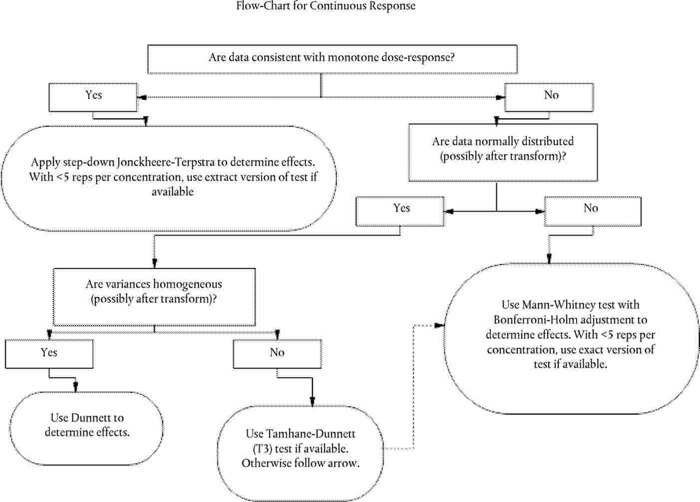
|
Special data analysis considerations
Use of compromised treatment levels
|
69.
|
Several factors are considered when determining whether a replicate or entire treatment demonstrates overt toxicity and should be removed from analysis. Overt toxicity is defined as > 2 mortalities in any replicate that can only be explained by toxicity rather than technical error. Other signs of overt toxicity include haemorrhage, abnormal behaviours, abnormal swimming patterns, anorexia and any other clinical signs of disease. For sub-lethal signs of toxicity, qualitative evaluations may be necessary, and should always be made in reference to the clean water control group.
|
Solvent controls
|
70.
|
The use of a solvent should only be considered as a last resort, when all other chemical delivery options have been considered. If a solvent is used, then a clean water control should be run in concert. At the termination of the test, an evaluation of the potential effects of the solvent should be performed. This is done through a statistical comparison of the solvent control group and the clean water control group. The most relevant endpoints for consideration in this analysis are developmental stage, SVL and wet weight, as these can be affected through non-thyroidal toxicities. If statistically significant differences are detected in these endpoints between the clean water control and solvent control groups, determine the study endpoints for the response measures using the clean water control. If there is no statistically significant difference between the clean water control and solvent control for all measured response variables, determine the study endpoints for the response measures using the pooled dilution-water and solvent controls.
|
Treatment groups achieving developmental stage 60 and above
|
71.
|
After stage 60, tadpoles show a reduction in size and weight due to tissue resorption and reduction of absolute water content. Thus, measurements of wet weight and SVL cannot appropriately be used in statistical analyses for differences in growth rates. Therefore, wet weight and length data from organisms > NF60 should be censored and cannot be used in analyses of replicate means or replicate medians. Two different approaches could be used to analyse these growth-related parameters.
|
|
72.
|
One approach is to consider only tadpoles with developmental stages lower or equal to stage 60 for the statistical analyses of wet weight and/or SVL. This approach is believed to provide sufficiently robust information about the severity of possible growth effects as long as only a small proportion of test animals are removed from the analyses (≤ 20 %). If an increased number of tadpoles show development beyond stage 60 (≥ 20 %) in one or more nominal concentration(s), then a two-factor ANOVA with a nested variance structure should be undertaken on all tadpoles to assess growth effects due to chemical treatments while taking into account the effect of late stage development on growth. Appendix 3 provides guidance on the two-factor ANOVA analysis of weight and length..
|
LITERATURE
|
(1)
|
OECD (2004) Report of the Validation of the Amphibian Metamorphosis Assay for the detection of thyroid active substances: Phase 1 — Optimisation of the Test Protocol. Environmental Health and Safety Publications. Series on Testing and Assessment. No. 77, Paris.
|
|
(2)
|
OECD (2007) Final Report of the Validation of the Amphibian Metamorphosis Assay: Phase 2 — Multi-chemical Interlaboratory Study. Environmental Health and Safety Publications. Series on Testing and Assessment. No. 76. Paris
|
|
(3)
|
OECD (2008) Report of the Validation Peer Review for the Amphibian Metamorphosis Assay and Agreement of the Working Group of the National Coordinators of the Test Guidelines Programme on the Follow-up of this Report. Environmental Health and Safety Publications. Series on Testing and Assessment. No. 92. Paris
|
|
(4)
|
OECD (2000) Guidance Document on Aquatic Toxicity Testing of Difficult Substances and Mixtures. Environmental Health and Safety Publications. Series on Testing and Assessment. No. 23. Paris
|
|
(5)
|
ASTM (2002) Standard Guide for Conducting Acute Toxicity Tests on Test Materials with Fishes, Macroinvertebrates, and Amphibians. American Society for Testing and Materials, ASTM E729-96(2002), Philadelpia, PA
|
|
(6)
|
ASTM (2004) Standard Guide for Conducting the Frog Embryo Teratogenesis Assay — Xenopus (FETAX). E 1439-98
|
|
(7)
|
Kahl,M.D., Russom,C.L., DeFoe,D.L. & Hammermeister,D.E. (1999) Saturation units for use in aquatic bioassays. Chemosphere 39, pp. 539-551
|
|
(8)
|
Nieuwkoop,P.D. & Faber,J. (1994) Normal Table of Xenopus laevis. Garland Publishing, New York
|
|
(9)
|
OECD (2007) Guidance Document on Amphibian Thyroid Histology. Environmental Health and Safety Publications. Series on Testing and Assessment. No. 82. Paris
|
|
(10)
|
Dodd,M.H.I. & Dodd,J.M. (1976) Physiology of Amphibia. Lofts,B. (ed.), Academic Press, New York, pp. 467-599
|
|
(11)
|
OECD (2006) Current Approaches in the Statistical Analysis of Ecotoxicity Data: A Guidance to Application. Environmental Health and Safety Publications. Series on Testing and Assessment, No. 54. Paris
|
|
(12)
|
Hutchinson TH, Shillabeer N, Winter MJ, Pickford DB, 2006. Acute and chronic effects of carrier solvents in aquatic organisms: A critical review. Review. Aquatic Toxicology, 76; pp.69–92.
|
Appendix 1
Table 1
Experimental Conditions for the 21-day Amphibian Metamorphosis Assay
|
Test Animal
|
Xenopus laevis larvae
|
|
Initial Larval Stage
|
Nieuwkoop and Faber stage 51
|
|
Exposure Period
|
21 days
|
|
Larvae Selection Criteria
|
Developmental stage and total length (optional)
|
|
Test Concentrations
|
Minimum of 3 concentrations spanning approximately one order of magnitude
|
|
Exposure Regime
|
Flow-through (preferred) and/or static-renewal
|
|
Test System Flow-Rate
|
25 ml/min (complete volume replacement ca. every 2,7 h)
|
|
Primary Endpoints/Determination Days
|
Mortality
|
Daily
|
|
Developmental Stage
|
D 7 and 21
|
|
Hind Limb Length
|
D 7 and 21
|
|
Snout-Vent Length
|
D 7 and 21
|
|
Wet Body Weight
|
D 7 and 21
|
|
Thyroid Histology
|
D 21
|
|
Dilution Water/Laboratory Control
|
Dechlorinated tap water (charcoal-filtered) or the equivalent laboratory source
|
|
Larval Density
|
20 larvae/test vessel (5/l)
|
|
Test Solution/Test Vessel
|
4-10 l (10-15 cm minimum water)/Glass or Stainless Steel test vessel (e.g., 22,5 cm × 14 cm × 16,5 cm)
|
|
Replication
|
4 replicate test vessels/test concentration and control
|
|
Acceptable Mortality Rate in Controls
|
≤ 10 % per replicate test vessel
|
|
Thyroid Fixation
|
Number Fixed
|
All tadpoles (5/replicate are evaluated initially)
|
|
Region
|
Head or whole body
|
|
Fixation Fluid
|
Davidson's fixative
|
|
Feeding
|
Food
|
Sera Micron® or equivalent
|
|
Amount/Frequency
|
See Table 1 for feeding regime using Sera Micron®
|
|
Lighting
|
Photoperiod
|
12 h Light: 12 h dark
|
|
Intensity
|
600 to 2 000 lux (Measured at Water Surface)
|
|
Water Temperature
|
22° ± 1 °C
|
|
pH
|
6,5 — 8,5
|
|
Dissolved Oxygen (DO) Concentration
|
> 3,5 mg/l (> 40 % Air Saturation)
|
|
Analytical Chemistry Sample Schedule
|
Once/Week (4 Sample Events/Test)
|
Appendix 2
Reporting tables for raw data and summary data
Table 1
General test chemical information
|
Chemical information
|
|
|
Enter test chemical, concentration units, and treatments
|
|
|
Test chemical:
|
|
|
|
|
Concentration units:
|
|
|
|
|
Treatment 1
|
|
|
|
|
Treatment 2
|
|
|
|
|
Treatment 3
|
|
|
|
|
Treatment 4
|
|
|
|
|
|
|
|
|
|
Date (day 0):
|
|
Enter date (mm/dd/yy)
|
|
|
Date (day 7):
|
|
Enter date (mm/dd/yy)
|
|
|
Date (day 21):
|
|
Enter date (mm/dd/yy)
|
Table 2
Raw data collection sheets for days 7 and 21
|
DAY X
DATE 00/00/00
|
|
|
Concentration
|
Treatment Number
|
Replicate Number
|
Individual number
|
Individual Idendifier
|
Developmental Stage
|
SVL Length (mm)
|
Hindlimb Length (mm)
|
Whole Organism wet weight (mg)
|
|
ROW
|
TRT
|
TRT#
|
REP
|
IND
|
ID#
|
STAGE
|
BL
|
HLL
|
WEIGHT
|
|
1
|
0,00
|
1
|
|
|
|
|
|
|
|
|
2
|
0,00
|
1
|
|
|
|
|
|
|
|
|
3
|
0,00
|
1
|
|
|
|
|
|
|
|
|
4
|
0,00
|
1
|
|
|
|
|
|
|
|
|
5
|
0,00
|
1
|
|
|
|
|
|
|
|
|
6
|
0,00
|
1
|
|
|
|
|
|
|
|
|
7
|
0,00
|
1
|
|
|
|
|
|
|
|
|
8
|
0,00
|
1
|
|
|
|
|
|
|
|
|
9
|
0,00
|
1
|
|
|
|
|
|
|
|
|
10
|
0,00
|
1
|
|
|
|
|
|
|
|
|
11
|
0,00
|
1
|
|
|
|
|
|
|
|
|
12
|
0,00
|
1
|
|
|
|
|
|
|
|
|
13
|
0,00
|
1
|
|
|
|
|
|
|
|
|
14
|
0,00
|
1
|
|
|
|
|
|
|
|
|
15
|
0,00
|
1
|
|
|
|
|
|
|
|
|
16
|
0,00
|
1
|
|
|
|
|
|
|
|
|
17
|
0,00
|
1
|
|
|
|
|
|
|
|
|
18
|
0,00
|
1
|
|
|
|
|
|
|
|
|
19
|
0,00
|
1
|
|
|
|
|
|
|
|
|
20
|
0,00
|
1
|
|
|
|
|
|
|
|
|
21
|
0,00
|
2
|
|
|
|
|
|
|
|
|
22
|
0,00
|
2
|
|
|
|
|
|
|
|
|
23
|
0,00
|
2
|
|
|
|
|
|
|
|
|
24
|
0,00
|
2
|
|
|
|
|
|
|
|
|
25
|
0,00
|
2
|
|
|
|
|
|
|
|
|
26
|
0,00
|
2
|
|
|
|
|
|
|
|
|
27
|
0,00
|
2
|
|
|
|
|
|
|
|
|
28
|
0,00
|
2
|
|
|
|
|
|
|
|
|
29
|
0,00
|
2
|
|
|
|
|
|
|
|
|
30
|
0,00
|
2
|
|
|
|
|
|
|
|
|
31
|
0,00
|
2
|
|
|
|
|
|
|
|
|
32
|
0,00
|
2
|
|
|
|
|
|
|
|
|
33
|
0,00
|
2
|
|
|
|
|
|
|
|
|
34
|
0,00
|
2
|
|
|
|
|
|
|
|
|
35
|
0,00
|
2
|
|
|
|
|
|
|
|
|
36
|
0,00
|
2
|
|
|
|
|
|
|
|
|
37
|
0,00
|
2
|
|
|
|
|
|
|
|
|
38
|
0,00
|
2
|
|
|
|
|
|
|
|
|
39
|
0,00
|
2
|
|
|
|
|
|
|
|
|
40
|
0,00
|
2
|
|
|
|
|
|
|
|
|
41
|
0,00
|
3
|
|
|
|
|
|
|
|
|
42
|
0,00
|
3
|
|
|
|
|
|
|
|
|
43
|
0,00
|
3
|
|
|
|
|
|
|
|
|
44
|
0,00
|
3
|
|
|
|
|
|
|
|
|
45
|
0,00
|
3
|
|
|
|
|
|
|
|
|
46
|
0,00
|
3
|
|
|
|
|
|
|
|
|
47
|
0,00
|
3
|
|
|
|
|
|
|
|
|
48
|
0,00
|
3
|
|
|
|
|
|
|
|
|
49
|
0,00
|
3
|
|
|
|
|
|
|
|
|
50
|
0,00
|
3
|
|
|
|
|
|
|
|
|
51
|
0,00
|
3
|
|
|
|
|
|
|
|
|
52
|
0,00
|
3
|
|
|
|
|
|
|
|
|
53
|
0,00
|
3
|
|
|
|
|
|
|
|
|
54
|
0,00
|
3
|
|
|
|
|
|
|
|
|
55
|
0,00
|
3
|
|
|
|
|
|
|
|
|
56
|
0,00
|
3
|
|
|
|
|
|
|
|
|
57
|
0,00
|
3
|
|
|
|
|
|
|
|
|
58
|
0,00
|
3
|
|
|
|
|
|
|
|
|
59
|
0,00
|
3
|
|
|
|
|
|
|
|
|
60
|
0,00
|
3
|
|
|
|
|
|
|
|
|
61
|
0,00
|
4
|
|
|
|
|
|
|
|
|
62
|
0,00
|
4
|
|
|
|
|
|
|
|
|
63
|
0,00
|
4
|
|
|
|
|
|
|
|
|
64
|
0,00
|
4
|
|
|
|
|
|
|
|
|
65
|
0,00
|
4
|
|
|
|
|
|
|
|
|
66
|
0,00
|
4
|
|
|
|
|
|
|
|
|
67
|
0,00
|
4
|
|
|
|
|
|
|
|
|
68
|
0,00
|
4
|
|
|
|
|
|
|
|
|
69
|
0,00
|
4
|
|
|
|
|
|
|
|
|
70
|
0,00
|
4
|
|
|
|
|
|
|
|
|
71
|
0,00
|
4
|
|
|
|
|
|
|
|
|
72
|
0,00
|
4
|
|
|
|
|
|
|
|
|
73
|
0,00
|
4
|
|
|
|
|
|
|
|
|
74
|
0,00
|
4
|
|
|
|
|
|
|
|
|
75
|
0,00
|
4
|
|
|
|
|
|
|
|
|
76
|
0,00
|
4
|
|
|
|
|
|
|
|
|
77
|
0,00
|
4
|
|
|
|
|
|
|
|
|
78
|
0,00
|
4
|
|
|
|
|
|
|
|
|
79
|
0,00
|
4
|
|
|
|
|
|
|
|
|
80
|
0,00
|
4
|
|
|
|
|
|
|
|
Table 3
Calculated summaries for endpoint data from days 7 and 21
|
|
|
Developmental Stage
|
SVL (mm)
|
Hindlimb Length (mm)
|
Weight (mg)
|
|
TRT
|
REP
|
MIN
|
MEDIAN
|
MAX
|
MEAN
|
STD DEV
|
MEAN
|
STD DEV
|
MEAN
|
STD DEV
|
|
1
|
1
|
0
|
#NUM!
|
0
|
#DIV/0!
|
#DIV/0!
|
#DIV/0!
|
#DIV/0!
|
#DIV/0!
|
#DIV/0!
|
|
1
|
2
|
0
|
#NUM!
|
0
|
#DIV/0!
|
#DIV/0!
|
#DIV/0!
|
#DIV/0!
|
#DIV/0!
|
#DIV/0!
|
|
1
|
3
|
0
|
#NUM!
|
0
|
#DIV/0!
|
#DIV/0!
|
#DIV/0!
|
#DIV/0!
|
#DIV/0!
|
#DIV/0!
|
|
1
|
4
|
0
|
#NUM!
|
0
|
#DIV/0!
|
#DIV/0!
|
#DIV/0!
|
#DIV/0!
|
#DIV/0!
|
#DIV/0!
|
|
2
|
1
|
0
|
#NUM!
|
0
|
#DIV/0!
|
#DIV/0!
|
#DIV/0!
|
#DIV/0!
|
#DIV/0!
|
#DIV/0!
|
|
2
|
2
|
0
|
#NUM!
|
0
|
#DIV/0!
|
#DIV/0!
|
#DIV/0!
|
#DIV/0!
|
#DIV/0!
|
#DIV/0!
|
|
2
|
3
|
0
|
#NUM!
|
0
|
#DIV/0!
|
#DIV/0!
|
#DIV/0!
|
#DIV/0!
|
#DIV/0!
|
#DIV/0!
|
|
2
|
4
|
0
|
#NUM!
|
0
|
#DIV/0!
|
#DIV/0!
|
#DIV/0!
|
#DIV/0!
|
#DIV/0!
|
#DIV/0!
|
|
3
|
1
|
0
|
#NUM!
|
0
|
#DIV/0!
|
#DIV/0!
|
#DIV/0!
|
#DIV/0!
|
#DIV/0!
|
#DIV/0!
|
|
3
|
2
|
0
|
#NUM!
|
0
|
#DIV/0!
|
#DIV/0!
|
#DIV/0!
|
#DIV/0!
|
#DIV/0!
|
#DIV/0!
|
|
3
|
3
|
0
|
#NUM!
|
0
|
#DIV/0!
|
#DIV/0!
|
#DIV/0!
|
#DIV/0!
|
#DIV/0!
|
#DIV/0!
|
|
3
|
4
|
0
|
#NUM!
|
0
|
#DIV/0!
|
#DIV/0!
|
#DIV/0!
|
#DIV/0!
|
#DIV/0!
|
#DIV/0!
|
|
4
|
1
|
0
|
#NUM!
|
0
|
#DIV/0!
|
#DIV/0!
|
#DIV/0!
|
#DIV/0!
|
#DIV/0!
|
#DIV/0!
|
|
4
|
2
|
0
|
#NUM!
|
0
|
#DIV/0!
|
#DIV/0!
|
#DIV/0!
|
#DIV/0!
|
#DIV/0!
|
#DIV/0!
|
|
4
|
3
|
0
|
#NUM!
|
0
|
#DIV/0!
|
#DIV/0!
|
#DIV/0!
|
#DIV/0!
|
#DIV/0!
|
#DIV/0!
|
|
4
|
4
|
0
|
#NUM!
|
0
|
#DIV/0!
|
#DIV/0!
|
#DIV/0!
|
#DIV/0!
|
#DIV/0!
|
#DIV/0!
|
|
Note: Cell calculations are associated with data entries into Table 2.
|
Table 4
Daily mortality data
|
Test Day
|
Date
|
1
|
2
|
3
|
4
|
1
|
2
|
3
|
4
|
1
|
2
|
3
|
4
|
1
|
2
|
3
|
4
|
|
0
|
00/00/00
|
|
|
|
|
|
|
|
|
|
|
|
|
|
|
|
|
|
1
|
#Value!
|
|
|
|
|
|
|
|
|
|
|
|
|
|
|
|
|
|
2
|
#Value!
|
|
|
|
|
|
|
|
|
|
|
|
|
|
|
|
|
|
3
|
#Value!
|
|
|
|
|
|
|
|
|
|
|
|
|
|
|
|
|
|
4
|
#Value!
|
|
|
|
|
|
|
|
|
|
|
|
|
|
|
|
|
|
5
|
#Value!
|
|
|
|
|
|
|
|
|
|
|
|
|
|
|
|
|
|
6
|
#Value!
|
|
|
|
|
|
|
|
|
|
|
|
|
|
|
|
|
|
7
|
#Value!
|
|
|
|
|
|
|
|
|
|
|
|
|
|
|
|
|
|
8
|
#Value!
|
|
|
|
|
|
|
|
|
|
|
|
|
|
|
|
|
|
9
|
#Value!
|
|
|
|
|
|
|
|
|
|
|
|
|
|
|
|
|
|
10
|
#Value!
|
|
|
|
|
|
|
|
|
|
|
|
|
|
|
|
|
|
11
|
#Value!
|
|
|
|
|
|
|
|
|
|
|
|
|
|
|
|
|
|
12
|
#Value!
|
|
|
|
|
|
|
|
|
|
|
|
|
|
|
|
|
|
13
|
#Value!
|
|
|
|
|
|
|
|
|
|
|
|
|
|
|
|
|
|
14
|
#Value!
|
|
|
|
|
|
|
|
|
|
|
|
|
|
|
|
|
|
15
|
#Value!
|
|
|
|
|
|
|
|
|
|
|
|
|
|
|
|
|
|
16
|
#Value!
|
|
|
|
|
|
|
|
|
|
|
|
|
|
|
|
|
|
17
|
#Value!
|
|
|
|
|
|
|
|
|
|
|
|
|
|
|
|
|
|
18
|
#Value!
|
|
|
|
|
|
|
|
|
|
|
|
|
|
|
|
|
|
19
|
#Value!
|
|
|
|
|
|
|
|
|
|
|
|
|
|
|
|
|
|
20
|
#Value!
|
|
|
|
|
|
|
|
|
|
|
|
|
|
|
|
|
|
21
|
#Value!
|
|
|
|
|
|
|
|
|
|
|
|
|
|
|
|
|
|
|
|
|
|
|
|
|
|
|
|
|
|
|
|
|
|
|
|
|
Replicate count
|
0
|
0
|
0
|
0
|
0
|
0
|
0
|
0
|
0
|
0
|
0
|
0
|
0
|
0
|
0
|
0
|
|
Treatment Count
|
0
|
|
|
|
0
|
|
|
|
0
|
|
|
|
0
|
|
|
|
|
Note: Cell calculations are associated with data entries into Table 1.
|
Table 5
Water Quality Criteria
Exposure System (flow-through/static renewal):
Temperature:
Light intensity:
Light-dark cycle:
Food:
Feeding rate:
water pH:
Iodine concentration in test water:
Table 6
Summary chemistry data
|
Chemical Name:
|
|
Cas #:
|
|
Test Day
|
Date
|
1
|
2
|
3
|
4
|
1
|
2
|
3
|
4
|
1
|
2
|
3
|
4
|
1
|
2
|
3
|
4
|
1
|
2
|
3
|
4
|
|
0
|
00/00/00
|
|
|
|
|
|
|
|
|
|
|
|
|
|
|
|
|
|
|
|
|
|
1
|
#Value!
|
|
|
|
|
|
|
|
|
|
|
|
|
|
|
|
|
|
|
|
|
|
2
|
#Value!
|
|
|
|
|
|
|
|
|
|
|
|
|
|
|
|
|
|
|
|
|
|
3
|
#Value!
|
|
|
|
|
|
|
|
|
|
|
|
|
|
|
|
|
|
|
|
|
|
4
|
#Value!
|
|
|
|
|
|
|
|
|
|
|
|
|
|
|
|
|
|
|
|
|
|
5
|
#Value!
|
|
|
|
|
|
|
|
|
|
|
|
|
|
|
|
|
|
|
|
|
|
6
|
#Value!
|
|
|
|
|
|
|
|
|
|
|
|
|
|
|
|
|
|
|
|
|
|
7
|
#Value!
|
|
|
|
|
|
|
|
|
|
|
|
|
|
|
|
|
|
|
|
|
|
8
|
#Value!
|
|
|
|
|
|
|
|
|
|
|
|
|
|
|
|
|
|
|
|
|
|
9
|
#Value!
|
|
|
|
|
|
|
|
|
|
|
|
|
|
|
|
|
|
|
|
|
|
10
|
#Value!
|
|
|
|
|
|
|
|
|
|
|
|
|
|
|
|
|
|
|
|
|
|
11
|
#Value!
|
|
|
|
|
|
|
|
|
|
|
|
|
|
|
|
|
|
|
|
|
|
12
|
#Value!
|
|
|
|
|
|
|
|
|
|
|
|
|
|
|
|
|
|
|
|
|
|
13
|
#Value!
|
|
|
|
|
|
|
|
|
|
|
|
|
|
|
|
|
|
|
|
|
|
14
|
#Value!
|
|
|
|
|
|
|
|
|
|
|
|
|
|
|
|
|
|
|
|
|
|
15
|
#Value!
|
|
|
|
|
|
|
|
|
|
|
|
|
|
|
|
|
|
|
|
|
|
16
|
#Value!
|
|
|
|
|
|
|
|
|
|
|
|
|
|
|
|
|
|
|
|
|
|
17
|
#Value!
|
|
|
|
|
|
|
|
|
|
|
|
|
|
|
|
|
|
|
|
|
|
18
|
#Value!
|
|
|
|
|
|
|
|
|
|
|
|
|
|
|
|
|
|
|
|
|
|
19
|
#Value!
|
|
|
|
|
|
|
|
|
|
|
|
|
|
|
|
|
|
|
|
|
|
20
|
#Value!
|
|
|
|
|
|
|
|
|
|
|
|
|
|
|
|
|
|
|
|
|
|
21
|
#Value!
|
|
|
|
|
|
|
|
|
|
|
|
|
|
|
|
|
|
|
|
|
|
Note: Cell calculations are associated with data entries into Table 1.
|
Table 7
Histopathology reporting tables for core criteria
|
Date:
|
Chemical:
|
|
|
Pathologist:
|
|
|
Thyroid gland hypertrophy
|
Thyroid gland atrophy
|
Follicular cell hypertrophy
|
Follicular cell hyperplasia
|
|
Thyroid gland hypertrophy
|
Thyroid gland atrophy
|
Follicular cell hypertrophy
|
Follicular cell hyperplasia
|
|
Control Animal ID — replicate 1
|
|
|
|
|
|
Dose Animal ID — replicate 1
|
|
|
|
|
|
|
|
|
|
|
|
|
|
|
|
|
|
|
|
|
|
|
|
|
|
|
|
|
|
|
|
|
|
|
|
|
|
|
|
|
|
|
|
|
|
|
|
|
|
|
Control Animal ID — replicate 2
|
|
|
|
|
|
Dose Animal ID — replicate 2
|
|
|
|
|
|
|
|
|
|
|
|
|
|
|
|
|
|
|
|
|
|
|
|
|
|
|
|
|
|
|
|
|
|
|
|
|
|
|
|
|
|
|
|
|
|
|
|
|
|
|
Total:
|
|
|
|
|
Total:
|
|
|
|
|
|
|
Thyroid gland hypertrophy
|
Thyroid gland atrophy
|
Follicular cell hypertrophy
|
Follicular cell hyperplasia
|
|
|
Thyroid gland hypertrophy
|
Thyroid gland atrophy
|
Follicular cell hypertrophy
|
Follicular cell hyperplasia
|
|
Dose Animal ID — replicate 1
|
|
|
|
|
|
Dose Animal ID — replicate 1
|
|
|
|
|
|
|
|
|
|
|
|
|
|
|
|
|
|
|
|
|
|
|
|
|
|
|
|
|
|
|
|
|
|
|
|
|
|
|
|
|
|
|
|
|
|
|
|
|
|
|
Dose Animal ID — replicate 2
|
|
|
|
|
|
Dose Animal ID — replicate 2
|
|
|
|
|
|
|
|
|
|
|
|
|
|
|
|
|
|
|
|
|
|
|
|
|
|
|
|
|
|
|
|
|
|
|
|
|
|
|
|
|
|
|
|
|
|
|
|
|
|
|
Total:
|
|
|
|
|
Total:
|
|
|
|
|
Table 8
Additional histopathology criteria
|
Date:
|
Chemical:
|
|
|
Pathologist:
|
|
|
|
|
|
|
|
|
Follicular lumen area increase
|
Follicular lumen area decrease
|
Follicular lumen area increase
|
Follicular lumen area decrease
|
|
Control Animal ID — replicate 1
|
|
|
|
Dose Animal ID — replicate 1
|
|
|
|
|
|
|
|
|
|
|
|
|
|
|
|
|
|
|
|
|
|
|
|
|
|
|
|
|
|
|
|
|
Control Animal ID — replicate 2
|
|
|
|
Dose Animal ID — replicate 2
|
|
|
|
|
|
|
|
|
|
|
|
|
|
|
|
|
|
|
|
|
|
|
|
|
|
|
|
|
|
|
|
|
Total:
|
|
|
Total:
|
|
|
|
|
Follicular lumen area increase
|
Follicular lumen area decrease
|
|
|
Follicular lumen area increase
|
Follicular lumen area decrease
|
|
Dose Animal ID — replicate 1
|
|
|
|
Dose Animal ID — replicate 1
|
|
|
|
|
|
|
|
|
|
|
|
|
|
|
|
|
|
|
|
|
|
|
|
|
|
|
|
|
|
|
|
|
Dose Animal ID — replicate 2
|
|
|
|
Dose Animal ID — replicate 2
|
|
|
|
|
|
|
|
|
|
|
|
|
|
|
|
|
|
|
|
|
|
|
|
|
|
|
|
|
|
|
|
|
Total:
|
|
|
Total:
|
|
|
Table 9
Narrative descriptions for histopathological findings
|
Date:
|
|
Chemical:
|
|
Pathologist:
|
|
|
Narrative description
|
|
Control Animal ID — replicate 1
|
|
|
|
|
|
|
|
|
|
|
|
|
|
|
|
Control Animal ID — replicate 2
|
|
|
|
|
|
|
|
|
|
|
|
|
|
|
|
|
|
Dose Animal ID — replicate 1
|
|
|
|
|
|
|
|
|
|
|
|
|
|
|
|
Dose Animal ID — replicate 2
|
|
|
|
|
|
|
|
|
|
|
|
|
|
|
|
|
|
Dose Animal ID — replicate 1
|
|
|
|
|
|
|
|
|
|
|
|
|
|
|
|
Dose Animal ID — replicate 2
|
|
|
|
|
|
|
|
|
|
|
|
|
|
|
|
|
|
|
|
Dose Animal ID — replicate 1
|
|
|
|
|
|
|
|
|
|
|
|
|
|
|
|
Dose Animal ID — replicate 2
|
|
|
|
|
|
|
|
|
|
|
|
|
|
|
Table 10
Summary reporting table template for day x (7 or 21) of the AMA
|
|
|
Control
|
Dose 1
|
Dose 2
|
Dose 3
|
|
Endpoint
|
Replicate
|
Mean
|
SD
|
CV
|
N
|
Mean
|
SD
|
CV
|
N
|
p-value
|
Mean
|
SD
|
CV
|
N
|
p-value
|
Mean
|
SD
|
CV
|
N
|
p-value
|
|
Hind Limb Length
(mm)
|
1
|
|
|
|
|
|
|
|
|
|
|
|
|
|
|
|
|
|
|
|
|
2
|
|
|
|
|
|
|
|
|
|
|
|
|
|
|
|
|
|
|
|
|
3
|
|
|
|
|
|
|
|
|
|
|
|
|
|
|
|
|
|
|
|
|
4
|
|
|
|
|
|
|
|
|
|
|
|
|
|
|
|
|
|
|
|
|
Mean:
|
|
|
|
|
|
|
|
|
|
|
|
|
|
|
|
|
|
|
|
|
SVL
(mm)
|
1
|
|
|
|
|
|
|
|
|
|
|
|
|
|
|
|
|
|
|
|
|
2
|
|
|
|
|
|
|
|
|
|
|
|
|
|
|
|
|
|
|
|
|
3
|
|
|
|
|
|
|
|
|
|
|
|
|
|
|
|
|
|
|
|
|
4
|
|
|
|
|
|
|
|
|
|
|
|
|
|
|
|
|
|
|
|
|
Mean:
|
|
|
|
|
|
|
|
|
|
|
|
|
|
|
|
|
|
|
|
|
Wet weight
(mg)
|
1
|
|
|
|
|
|
|
|
|
|
|
|
|
|
|
|
|
|
|
|
|
2
|
|
|
|
|
|
|
|
|
|
|
|
|
|
|
|
|
|
|
|
|
3
|
|
|
|
|
|
|
|
|
|
|
|
|
|
|
|
|
|
|
|
|
4
|
|
|
|
|
|
|
|
|
|
|
|
|
|
|
|
|
|
|
|
|
Mean:
|
|
|
|
|
|
|
|
|
|
|
|
|
|
|
|
|
|
|
|
Table 11
Summary reporting table template for day x (7 or 21) developmental stage data for the AMA
|
|
|
Control
|
Dose 1
|
Dose 2
|
Dose 3
|
|
|
Replicate
|
Median
|
Min
|
Max
|
N
|
Median
|
Min
|
Max
|
N
|
p-value
|
Median
|
Min
|
Max
|
N
|
p-value
|
Median
|
Min
|
Max
|
Median
|
p-value
|
|
Developmental Stage
|
1
|
|
|
|
|
|
|
|
|
|
|
|
|
|
|
|
|
|
|
|
|
2
|
|
|
|
|
|
|
|
|
|
|
|
|
|
|
|
|
|
|
|
|
3
|
|
|
|
|
|
|
|
|
|
|
|
|
|
|
|
|
|
|
|
|
4
|
|
|
|
|
|
|
|
|
|
|
|
|
|
|
|
|
|
|
|
|
Mean:
|
|
|
|
|
|
|
|
|
|
|
|
|
|
|
|
|
|
|
|
Appendix 3
Alternative Analysis of weight and length in the case of late stage development exceeding 20 % of tadpoles in one or more concentration(s)
If an increased number of tadpoles show development beyond stage 60 (≥ 20 %) in one or more nominal concentration(s), then a two-factor ANOVA with a nested variance structure should be undertaken on all tadpoles to assess growth effects due to chemical treatments while taking into account the effect of late stage development on growth.
The proposal is to use all data but take into account the effect of late stage development. This can be done with a two-factor ANOVA with a nested variance structure. Define LateStage = ’Yes’ for an animal if its developmental stage is 61 or greater. Otherwise, define LateStage = ’No’. Then a two-factor ANOVA with concentration and LateStage and their interaction can be done, with Rep(Conc) a random factor and Tadpole(Rep) another random effect. This still treats the rep as the unit of analysis and gives essentially the same results as a weighted analysis of rep*latestage means, weighted by the number of animals per mean. If the data violate the normality or variance homogeneity requirements of ANOVA, then a normalised rank-order transform can be done to remove that objection.
In addition to the standard ANOVA F-tests for the effects of Conc, LateStage, and their interactions, the interaction F-test can be “sliced” into two additional ANOVA F-test, one on the mean responses across concentrations for LateStage = ’No’ and another on the mean responses across concentrations for LateStage = ’Yes’. Further comparisons of treatment means against control are done within each level of LateStage. A trend-type analysis can be done using appropriate contrasts or simple pairwise comparisons can be done if there is evidence of non-monotone dose-response within a level of the LateStage variable. A Bonferroni-Holm adjustment to the p-values is made only if the corresponding F-slice is not significant. This can be done in SAS and, presumably, other statistical software packages. Complications can arise when there are no late stage animals in some concentrations, but these situations can be handled in a straight-forward fashion.
Appendix 4
Definitions
Chemical
: A substance or a mixture
Test chemical
: Any substance or mixture tested using this test method
C.39. COLLEMBOLAN REPRODUCTION TEST IN SOIL
INTRODUCTION
|
1.
|
This test method is equivalent to OECD test guideline (TG) 232 (2009). This test method is designed for assessing the effects of chemicals on the reproductive output of the collembolans in soil. It is based on existing procedures (1) (2). The parthenogenetic Folsomia candida and sexually reproducing Folsomia fimetaria are two of the most accessible species of Collembola, and they are culturable and commercially available. When specific habitats not covered by the two species need to be assessed the procedure is extensible also to other species of Collembola if they are able to fulfil the validity criteria of the test.
|
|
2.
|
Soil-dwelling Collembola are ecologically relevant species for ecotoxicological testing. Collembolans are hexapods with a thin exoskeleton highly permeable to air and water, and represent arthropod species with a different route and a different rate of exposure compared to earthworms and enchytraeids.
|
|
3.
|
Population densities of Collembola commonly reach 105 m– 2 in soil and leaf litter layers in many terrestrial ecosystems (3) (4). Adults typically measure 0,5 - 5 mm, their contribution to total soil animal biomass and respiration is low, estimated between 1 % and 5 % (5). Their most important role may therefore be as potential regulators of processes through microbivory and microfauna predation. Springtails are prey animals for a wide variety of endogeic and epigeic invertebrates, such as mites, centipedes, spiders, Carabidae and rove beetles. Collembola contribute to decomposition processes in acidic soils where they may be the most important soil invertebrates besides enchytraeids, since earthworms and diplopods are typically absent.
|
|
4.
|
F. fimetaria has a worldwide distribution and is common in several soil types ranging from sandy to loamy soils and from mull to mor soils. It is an eyeless, unpigmented collembolan. It has been recorded in agricultural soils all over Europe (6). It has an omnivorous feeding habit, including fungal hyphae, bacteria, protozoa and detritus in its food. It interacts through grazing with infections of plant pathogenic fungi (7) and may influence mycorrhiza, as is known to be the case for F. candida. As most collembolan species it reproduces sexually requiring the permanent presence of males for egg fertilisation.
|
|
5.
|
F. candida is also distributed worldwide. Although it is not common in most natural soils, it often occurs in very high numbers in humus rich sites. It is an eyeless, unpigmented collembolan. It has a well-developed furca (jumping organ) and an active running movement and jumps readily if disturbed. The ecological role of F. candida is similar to the role of F. fimetaria, but the habitats are more organic rich soils. It reproduces parthenogenetically. Males may occur at less than 1 per thousand.
|
PRINCIPLE OF THE TEST
|
6.
|
Synchronous adult (F. fimetaria) or juvenile (F. candida) Collembola are exposed to a range of concentrations of the test chemical mixed into a modified artificial soil (8) using a 5 % organic matter content (or an alternative soil). The test scenario can be divided into two steps:
|
—
|
A range-finding test, in case no sufficient information on toxicity is available, in which mortality and reproduction are the main endpoints assessed after 2 weeks for F. fimetaria and 3 weeks for F. candida.
|
|
—
|
A definitive reproduction test in which the total number of juveniles produced by parent animals and the survival of parent animals are assessed. The duration of this definitive test is 3 weeks for F. fimetaria or 4 weeks for F. candida.
|
The toxic effect of the test chemical on adult mortality and reproductive output is expressed as LCx and ECx by fitting the data to an appropriate model by non-linear regression to estimate the concentration that would cause x % mortality or reduction in reproductive output, respectively, or alternatively as the NOEC/LOEC value (9).
|
INFORMATION ON THE TEST CHEMICAL
|
7.
|
The physical properties, water solubility, the log Kow, the soil water partition coefficient and the vapour pressure of the test chemical should preferably be known. Additional information on the fate of the test chemical in soil, such as the rates of photolysis and hydrolysis and biotic degradation, is desirable. Chemical identification of the test chemical according to IUPAC nomenclature, CAS-number, batch, lot, structural formula and purity should be documented when available.
|
|
8.
|
This Test Method can be used for water soluble or insoluble chemicals. However, the mode of application of the test chemical will differ accordingly. The test method is not applicable to volatile chemicals, i.e. chemicals for which the Henry's constant or the air/water partition coefficient is greater than one, or chemicals for which the vapour pressure exceeds 0,0133 Pa at 25 °C.
|
VALIDITY OF THE TEST
|
9.
|
The following criteria should be satisfied in the untreated controls for a test result to be considered valid:
|
—
|
Mean adult mortality should not exceed 20 % at the end of the test;
|
|
—
|
The mean number of juveniles per vessel should be at least 100 at the end of the test;
|
|
—
|
The coefficient of variation calculated for the number of juveniles should be less than 30 % at the end of the definitive test.
|
|
REFERENCE CHEMICAL
|
10.
|
A reference chemical should be tested at its EC50 concentration for the chosen test soil type either at regular intervals or possibly included in each test run to verify that the response of the test organisms in the test system are within the normal level. A suitable reference chemical is boric acid, which should reduce reproduction by 50 % (10) (11) at about 100 mg/kg dry weight soil for both species.
|
DESCRIPTION OF THE TEST
Test vessels and equipment
|
11.
|
Containers capable of holding 30 g of moist soil are suitable test vessels. The material should either be glass or inert plastic (non-toxic). However, using plastic containers should be avoided if the test chemical exposure is decreased due to sorption. The test vessels should have a cross-sectional area allowing the actual soil depth within the test vessel to be 2-4 cm. The vessels should have lids (e.g. glass or polyethylene) that are designed to reduce water evaporation whilst allowing gas exchange between the soil and the atmosphere. The container should be at least partly transparent to allow light transmission.
|
|
12.
|
Normal laboratory equipment is required, specifically the following:
|
—
|
suitable accurate balances;
|
|
—
|
adequate equipment for temperature control;
|
|
—
|
adequate equipment for air humidity control (not essential if exposure vessels are covered by lids);
|
|
—
|
temperature-controlled incubator or small room;
|
|
—
|
forceps or a low-suction air flow device.
|
|
Preparation of the test soil
|
13.
|
A modified artificial soil (8) is used with an organic matter content of 5 %. Alternatively a natural soil could be used, as the artificial soil does not resemble natural soils. The recommended composition of the artificial soil is as follows (based on dry weights, dried to a constant weight at 105 °C):
|
—
|
5 % sphagnum peat, air-dried and finely ground (a particle size of 2 ± 1 mm is acceptable);
|
|
—
|
20 % kaolin clay (kaolinite content preferably above 30 %);
|
|
—
|
approximately 74 % air-dried industrial sand (depending on the amount of CaCO3 needed), predominantly fine sand with more than 50 % of the particles between 50 and 200 microns. The exact amount of sand depends on the amount of CaCO3 (see below), together they should add up to 75 %.
|
|
—
|
1,0 % calcium carbonate (CaCO3, pulverised, analytical grade) to obtain a pH of 6,0 ± 0,5; the amount of calcium carbonate to be added may depend principally on the quality/nature of the peat (see Note 1).
|
Note 1: The amount of CaCO3 required will depend on the components of the soil substrate and should be determined by measuring the pH of pre-incubated moist soil sub-samples immediately before the test.
Note 2: It is recommended to measure the pH and optionally the C/N ratio, Cation Exchange Capacity (CEC) and organic matter content of the soil in order to enable a normalisation at a later stage and to better interpret the results.
Note 3: If required, e.g. for specific testing purposes, natural soils from unpolluted sites may also serve as test and/or culture substrate. However, if natural soil is used, it should be characterised at least by origin (collection site), pH, texture (particle size distribution), CEC and organic matter content and it should be free from any contamination. For natural soil it is advisable to demonstrate its suitability for a test and for achieving the test validity criteria before using the soil in a definitive test.
|
|
14.
|
The dry constituents of the soil are mixed thoroughly (e.g. in a large-scale laboratory mixer). The maximum water holding capacity (WHC) of the artificial soil is determined in accordance with procedures described in Appendix 5. The moisture content of the testing soil should be optimised to attain a loose porous soil structure allowing collembolans to enter into the pores. This is usually between 40-60 % of the maximum WHC.
|
|
15.
|
The dry artificial soil is pre-moistened by adding enough de-ionised water to obtain approximately half of the final water content 2-7 days before the test start, in order to equilibrate/stabilise the acidity. For the determination of pH a mixture of soil and 1 M potassium chloride (KCl) or 0,01 M calcium chloride (CaCl2) solution in a 1:5 ratio is used (according to Appendix 6). If the soil is more acidic than the required range, it can be adjusted by addition of an appropriate amount of CaCO3. If the soil is too alkaline it can be adjusted by the addition of an inorganic acid harmless to collembolans.
|
|
16.
|
The pre-moistened soil is divided into portions corresponding to the number of test concentrations (and reference chemical where appropriate) and controls used for the test. The test chemicals are added and the water content is regulated according to the paragraph 24.
|
Selection and preparation of test animals
|
17.
|
The parthenogenetic F. candida is the recommended species, as in the ring testing of the test method (11) this species met the validity criteria for survival more often than F. fimetaria. If an alternative species is used, it should meet the validity criteria outlined in paragraph 9. At the start of the test the animals should be well fed and the age between 23-26 days for F. fimetaria and 9-12 days for F. candida. For each replicate, the number of F. fimetaria should be 10 males and 10 females, and for F. candida 10 females should be used (see Appendix 2 and Appendix 3). The synchronous animals are selected randomly from the dishes and their health and physical condition is checked for each batch added to a replicate. Each group of 10/20 individuals is added to a randomly selected test container and the big females of F. fimetaria are selected to ensure a proper distinction from the F. fimetaria males.
|
Preparation of test concentrations
|
18.
|
Four methods of application of the test chemical can be used: 1) mixing the test chemical into the soil with water as a carrier, 2) mixing the test chemical into the soil with an organic solvent as a carrier, 3) mixing the test chemical into the soil with sand as a carrier, or 4) application of the test chemical onto the soil surface. The selection of the appropriate method depends on the characteristic of the chemical and the purpose of the test. In general, mixing of the test chemical into the soil is recommended. However, application procedures that are consistent with the practical use of the test chemical may be required (e.g. spraying of liquid formulation or use of special pesticide formulations such as granules or seed dressings). The soil is treated before the collembolans are added, except when the test chemical is added to the soil surface collembolans should be allowed to enter the soil.
|
Test chemical soluble in water
|
19.
|
A solution of the test chemical is prepared in deionised water in a quantity sufficient for all replicates of one test concentration. Each solution of test chemical is mixed thoroughly with one batch of pre-moistened soil before being introduced into the test vessel.
|
Test chemical insoluble in water
|
20.
|
For chemicals insoluble in water, but soluble in organic solvents, the test chemical can be dissolved in the smallest possible volume of a suitable solvent (e.g. acetone) still ensuring proper mixing of the chemical in the soil and mixing it with a portion of the quartz sand required. Only volatile solvents should be used. When an organic solvent is used, all test concentrations and an additional solvent negative control should contain the same minimum amount of the solvent. Application containers should be left uncovered for a certain period to allow the solvent associated with the application of the test chemical to evaporate, ensuring no dissipation of the toxic chemical during this time.
|
Test chemical poorly soluble in water and organic solvents
|
21.
|
For chemicals that are poorly soluble in water and organic solvents, quartz sand, which should be a part of the total sand added to the soil, is mixed with the quantity of test chemical to obtain the desired test concentration. This mixture of quartz sand and test chemical is added to the pre-moistened soil and thoroughly mixed after adding an appropriate amount of deionised water to obtain the required moisture content. The final mixture is divided between the test vessels. The procedure is repeated for each test concentration and an appropriate control is also prepared.
|
Application of the test chemical onto the soil surface
|
22.
|
When the test chemical is a pesticide, it may be appropriate to apply it onto the soil surface by spraying. The soil is treated after the collembolans are added. The test containers are first filled with the moistened soil substrate, and the animals added and then the test containers are weighted. In order to avoid any direct exposure of the animals with the test chemical by direct contact, the test chemical is applied at least half an hour after introducing the Collembola. The test chemical should be applied to the surface of the soil as evenly as possible using a suitable laboratory-scale spraying device to simulate spray application in the field. The application should take place at a temperature within ± 2 °C of variation and for aqueous solutions, emulsions or dispersions at a water application rate according to the risk assessment recommendations. The rate should be verified using an appropriate calibration technique. Special formulations like granules or seed dressings could be applied in a manner consistent with agricultural use. Food is added after spraying.
|
PROCEDURE
Test conditions
|
23.
|
The test mean temperature should be 20 ± 1 °C with a temperature range of 20 ± 2 °C. The test is carried out under controlled light-dark cycles (preferably 12 hours light and 12 hours dark) with illumination of 400 to 800 lux in the area of the test vessels.
|
|
24.
|
In order to check the soil humidity, the vessels are weighed at the beginning, in the middle and at the end of the test. Weight loss > 2 % is replenished by the addition of de-ionised water. It should be noted that loss of water can be reduced by maintaining a high air-humidity (> 80 %) in the test incubator.
|
|
25.
|
The pH should be measured at the beginning and the end of both the range-finding test and the definitive test. Measurements should be made in one extra control sample and one extra sample of the treated (all concentrations) soil samples prepared and maintained in the same way as the test cultures, but without addition of the collembolans.
|
Test procedure and measurements
|
26.
|
For each test concentration, an amount of test soil corresponding to 30 g fresh weight is placed into the test vessel. Water controls, without the test chemical, are also prepared. If a vehicle is used for application of the test chemical, one control series containing the vehicle alone should be run in addition to the test series. The solvent or dispersant concentration should be the same as that used in the test vessels containing the test chemical.
|
|
27.
|
The individual springtails are carefully transferred into each test vessel (allocated randomly to the test vessels) and placed onto the surface of the soil. For efficient transfer of the animals, a low-suction air flow device can be used. The number of replicates for test concentrations and for controls depends on the test design used. The test vessels are positioned randomly in the test incubator and these positions are re-randomised weekly.
|
|
28.
|
For the F. fimetaria test twenty adults, 10 males and 10 females, 23-26 days old should be used per test-vessel. On day 21 collembolans are extracted from the soil and counted. For F. fimetaria the gender are discriminated by size in the synchronised animal batch used for the test. Females are distinctively larger than the males (See Appendix 3)
|
|
29.
|
For the F. candida test, ten 9-12 days old juveniles per test vessel should be used. On day 28, the collembolans are extracted from the soil and counted.
|
|
30.
|
As a suitable food source, a sufficient amount, e.g. 2-10 mg, of granulated dried baker's yeast, commercially available for household use, is added to each container at the beginning of the test and after about 2 weeks.
|
|
31.
|
At the end of the test, mortality and reproduction are assessed. After 3 weeks (F. fimetaria) or 4 weeks (F. candida), collembolans are extracted from the test soil (see Appendix 4) and counted (12). A collembolan is recorded as dead if not present in the extraction. The extraction and counting method should be validated. The validity includes extraction efficiency of juveniles greater than 95 %, e.g. by adding a known number to soil.
|
|
32.
|
Practical summary and timetable of the test procedure are described in Appendix 2.
|
Test design
Range-finding test
|
33.
|
When necessary, a range-finding test is conducted with, for example, five test chemical concentrations of 0,1, 1,0, 10, 100, and 1 000 mg/kg dry weight of soil and two replicates for each treatment and control. Additional information, from tests with similar chemicals or from literature, on mortality or reproduction of Collembola may also be useful in deciding on the range of concentrations to be used in the range-finding test.
|
|
34.
|
The duration of the range-finding test is two weeks for F. fimetaria and 3 weeks for F. candida to ensure one clutch of juveniles has been produced. At the end of the test, mortality and reproduction of the Collembola are assessed. The number of adults and the occurrence of juveniles should be recorded.
|
Definitive test
|
35.
|
For determination of the ECx (e.g. EC10, EC50), twelve concentrations should be tested. At least two replicates for each test concentration treatment and six control replicates are recommended. The spacing factor may vary depending on the dose-response pattern.
|
|
36.
|
For determination of the NOEC/LOEC, at least five concentrations in a geometric series should be tested. Four replicates for each test concentration treatment plus eight controls are recommended. The concentrations should be spaced by a factor not exceeding 1,8.
|
|
37.
|
A combined approach allows for determination of both the NOEC/LOEC and ECx. For this combined approach, eight treatment concentrations in a geometric series should be used. Four replicates for each treatment plus eight controls are recommended. The concentrations should be spaced by a factor not exceeding 1,8.
|
|
38.
|
If no effects are observed at the highest concentration in the range-finding test (i.e. 1 000 mg/kg), the reproduction test can be performed as a limit test, using a test concentration of 1 000 mg/kg and the control. A limit test will provide the opportunity to demonstrate that there is no statistically significant effect at the limit concentration. Eight replicates should be used for both the treated soil and the control.
|
DATA AND REPORTING
Treatment of results
|
39.
|
The reproductive output is the main endpoint (e.g. the number of juveniles produced per test vessel). The statistical analysis, e.g. ANOVA procedures, compares treatments by Student t-test, Dunnett's test, or Williams' test. 95 % confidence intervals are calculated for individual treatment means.
|
|
40.
|
The number of surviving adults in the untreated controls is a major validity criterion and should be documented. As in the range-finding test, all other harmful signs should be reported in the final report as well.
|
LCx and ECx
|
41.
|
ECx-values, including their associated lower and upper 95 % confidence limits for the parameter, are calculated using appropriate statistical methods (e.g. logistic or Weibull function, trimmed Spearman-Karber method, or simple interpolation). An ECx is obtained by inserting a value corresponding to x % of the control mean into the equation found. To compute the EC50 or any other ECx, the complete data set should be subjected to regression analysis. LC50 is usually estimated by probit analysis or similar analysis that takes into account the binomially distributed mortality data.
|
NOEC/LOEC
|
42.
|
If a statistical analysis is intended to determine the NOEC/LOEC, per-vessel statistics (individual vessels are considered replicates) are necessary. Appropriate statistical methods should be used according to OECD Document 54 on the Current Approaches in the Statistical Analysis of Ecotoxicity Data: a Guidance to Application (9). In general, adverse effects of the test chemical compared to the control are investigated using one-tailed hypothesis testing at p ≤ 0,05.
|
|
43.
|
Normal distribution and variance homogeneity can be tested using an appropriate statistical test, e.g. the Shapiro-Wilk test and Levene test, respectively (p ≤ 0,05). One-way Analysis of Variance (ANOVA) and subsequent multi-comparison tests can be performed. Multiple comparisons (e.g. Dunnett's test) or step-down trend tests (e.g. Williams' test) can be used to calculate whether there are significant differences (p ≤ 0,05) between the controls and the various test chemical concentrations (selection of the recommended test according to OECD Document 54 (9)). Otherwise, non-parametric methods (e.g. Bonferroni-U-test according to Holm or Jonckheere-Terpstra trend test) could be used to determine the NOEC and the LOEC.
|
Limit test
|
44.
|
If a limit test (comparison of control and one treatment only) has been performed and the prerequisites of parametric test procedures (normality, homogeneity) are fulfilled, metric responses can be evaluated by the Student test (t-test). The unequal-variance t-test (Welch t-test) or a non parametric test, such as the Mann-Whitney-U-test may be used, if these requirements are not fulfilled.
|
|
45.
|
To determine significant differences between the controls (control and solvent control), the replicates of each control can be tested as described for the limit test. If these tests do not detect significant differences, all control and solvent control replicates may be pooled. Otherwise all treatments should be compared with the solvent control.
|
Test report
|
46.
|
The test report should at least include the following information:
|
|
Test chemical
|
—
|
the identity of the test chemical, batch, lot and CAS-number, purity;
|
|
—
|
physico-chemical properties of the test chemical (e.g. log Kow, water solubility, vapour pressure, Henry's constant (H) and preferably information on the fate of the test chemical in soil) if available;
|
|
—
|
the formulation of the test chemical and the additives should be specified if not the pure chemical is tested;
|
|
|
|
Test organisms
|
—
|
identification of species and supplier of the test organisms, description of the breeding conditions and age range of test organisms;
|
|
|
|
Test conditions
|
—
|
description of the experimental design and procedure;
|
|
—
|
preparation details for the test soil; detailed specification if natural soil is used (origin, history, particle size distribution, pH, organic matter content);
|
|
—
|
water holding capacity of the soil;
|
|
—
|
description of the technique used to apply the test chemical to the soil;
|
|
—
|
test conditions: light intensity, duration of light-dark cycles, temperature;
|
|
—
|
a description of the feeding regime, the type and amount of food used in the test, feeding dates;
|
|
—
|
pH and water content of the soil at the start and end of the test (control and each treatment);
|
|
—
|
detailed description of the extraction method and extraction efficiency;
|
|
|
|
Test results
|
—
|
the number of juveniles determined in each test vessel at the end of the test;
|
|
—
|
number of adults and their mortality (%) in each test vessel at the end of the test;
|
|
—
|
a description of obvious physiological or pathological symptoms or distinct changes in behaviour;
|
|
—
|
the results obtained with the reference test chemical;
|
|
—
|
the NOEC/LOEC values, LCx for mortality and ECx for reproduction (mostly LC50, LC10, EC50, and EC10) together with 95 % confidence intervals. A graph of the fitted model used for calculation, its function equation and its parameters (See (9));
|
|
—
|
all information and observations helpful for the interpretation of the results;
|
|
—
|
power of the actual test if hypothesis testing is done (9);
|
|
—
|
deviations from procedures described in this Test Method and any unusual occurrences during the test;
|
|
—
|
for NOEC, when estimated, the minimal detectable difference.
|
|
|
LITERATURE
|
(1)
|
Wiles JA and Krogh PH (1998) Testing with the collembolans I. viridis, F. candida and F. fimetaria. In Handbook of soil invertebrate toxicity tests (ed. H Løkke and CAM Van Gestel), pp. 131-156. John Wiley & Sons, Ltd., Chichester
|
|
(2)
|
ISO (1999) Soil Quality — Effects of soil pollutants on Collembola (Folsomia candida): Method for determination of effects on reproduction. No. 11267. International Organisation for Standardisation, Geneve
|
|
(3)
|
Burges A and Raw F (Eds) (1967) Soil Biology. Academic Press. London
|
|
(4)
|
Petersen H and Luxton M (1982) A comparative analysis of soil fauna populations and their role in decomposition processes. Oikos 39: 287-388
|
|
(5)
|
Petersen H (1994) A review of collembolan ecology in ecosystem context. Acta Zoologica Fennica 195: 111-118
|
|
(6)
|
Hopkin SP (1997). Biology of the Springtails (Insecta: Collembola). Oxford University Press. 330pp (ISBN 0-19-854084-1)
|
|
(7)
|
Ulber B (1983) Einfluss von Onychirurus fimatus Gisin (Collembola, Onychiuridae) und Folsomia fimetaria L. (Collembola, Isotomidae) auf Pythium ultimum Trow. einen Erreger des Wurzelbrandes der Zuckerrübe. In New trends in soil Biology (Lebrun Ph, André HM, De Medts A, Grégoire-Wibo, Wauthy G (Eds), Proceedings of the VI. international colloquium on soil zoology, Louvain-la-neuve (Belgium), 30 August-2 September 1982, I Dieu-Brichart, Ottignies-Louvain-la-Neuve, pp. 261-268
|
|
(8)
|
Chapter C.36 of this Annex, Predatory mite (Hypoaspis (Geolaelaps) aculeifer) reproduction test in soil.
|
|
(9)
|
OECD (2006), Current approaches in the statistical analysis of ecotoxicity data: a guidance to application. OECD series on testing and assessment Number 54, ENV/JM/MONO(2006)18, OECD Paris
|
|
(10)
|
Scott-Fordsmand JJ and Krogh PH (2005) Background report on prevalidation of an OECD springtail test guideline. Environmental Project Nr. 986. Miljøstyrelsen 61 pp. Danish Ministry for the Environment.
|
|
(11)
|
Krogh, P.H., 2009. Toxicity testing with the collembolans Folsomia fimetaria and Folsomia candida and the results of a ringtest. Danish Environmental Protection Agency, Environmental Project No. 1256, pp. 66.
|
|
(12)
|
Krogh PH, Johansen K and Holmstrup M (1998) Automatic counting of collembolans for laboratory experiments. Appl. Soil Ecol. 7, 201-205
|
|
(13)
|
Fjellberg A (1980) Identification keys to Norwegian collembolans. Norsk Entomologisk Forening.
|
|
(14)
|
Edwards C.A. (1955) Simple techniques for rearing Collembola, Symphyla and other small soil inhabiting arthropods. In Soil Zoology (Kevan D.K. McE., Ed). Butterworths, London, pp. 412-416
|
|
(15)
|
Goto HE (1960) Simple techniques for the rearing of Collembola and a not on the use of a fungistatic substance in the cultures. Entomologists' Monthly Magazine 96:138-140.
|
Appendix 1
Definitions
The following definitions are applicable to this test method (in this test all effect concentrations are expressed as a mass of test chemical per dry mass of the test soil):
|
|
Chemical is a substance or a mixture.
|
|
|
NOEC (no observed effect concentration) is the test chemical concentration at which no effect is observed. In this test, the concentration corresponding to the NOEC, has no statistically significant effect (p < 0,05) within a given exposure period when compared with the control.
|
|
|
LOEC (lowest observed effect concentration) is the lowest test chemical concentration that has a statistically significant effect (p < 0,05) within a given exposure period when compared with the control.
|
|
|
ECx (Effect concentration for x % effect) is the concentration that causes an x % of an effect on test organisms within a given exposure period when compared with a control. For example, an EC50 is a concentration estimated to cause an effect on a test end point in 50 % of an exposed population over a defined exposure period.
|
|
|
Test chemical is any substance or mixture tested using this test method.
|
Appendix 2
Main actions and timetable for performing a collembolan test
The steps of the test can be summarised as follows:
|
Time (day)
|
Action
|
|
– 23 to – 26
|
Preparation of synchronous F. fimetaria culture
|
|
– 14
|
Prepare artificial soil (mixing of dry constituents)
Check pH of artificial soil and adjust accordingly
Measure max WHC of soil
|
|
– 9 to – 12
|
Preparation of synchronous F. candida culture
|
|
– 2 to – 7
|
Pre-moist soil
|
|
– 1
|
Distribute juveniles into batches
Prepare stock solutions and apply test chemical if solvent required
|
|
0
|
Prepare stock solutions and apply test chemical if solid chemical, water soluble or surface application is required.
Measure soil pH and weigh the containers.
Add food. Introduce collembolans.
|
|
14
|
Range-finding test F. fimetaria: Terminate test, extract animals, measure soil pH and loss of water (weight)
Definitive tests: Measure moisture content and replenish water and add 2-10 mg yeast
|
|
21
|
Definitive F. fimetaria test: Terminate test, extract animals, measure soil pH and loss of water (weight)
Range-finding F. candida: Terminate test, extract animals, measure soil pH and loss of water (weight)
|
|
28
|
Definitive F. candida test: Terminate test, extract animals, measure soil pH and loss of water (weight)
|
Appendix 3
Guidance on rearing and synchronisation of F. fimetaria and F. candida
The time and durations given in this guidance should be checked for each specific collembolan strain to ensure that timing will allow for sufficient synchronised juveniles. Basically, the incidence of oviposition after the adults are transferred to fresh substrate and egg hatching determines the appropriate day for egg collection and collection of synchronous juveniles.
It is recommended to have a permanent stock culture consisting of e.g. 50 containers/Petri dishes. The stock culture should be kept in a good feeding condition by weekly feeding, watering and removal of old food and carcasses. Too few collembolans on the substrate may result in inhibition by more fungal growth. If the stock culture is used for egg production too often, the culture may get fatigue. Signs of fatigue are dead adults and mould on the substrate. The remaining eggs from the production of synchronous animals can be used to rejuvenate the culture.
In a synchronous culture of F. fimetaria, males are distinguished from females primarily by size. Males are clearly smaller than females, and the walking speed of the males is faster than for females. Correct selection of the gender requires little practice and can be confirmed by microscopic inspection of the genital area (13).
1. Rearing
1.a. Preparation of culturing substrate
The culturing substrate is plaster of Paris (calcium sulphate) with activated charcoal. This provides a moist substrate, with the function of the charcoal being to absorb waste gases and excreta (14) (15). Different forms of charcoal may be used to facilitate observations of the Collembola. For example, powdered charcoal is used for F. candida and F. fimetaria (producing a black/grey plaster of Paris):
Substrate constituents:
|
—
|
20 ml of activated charcoal
|
|
—
|
200 ml of distilled water
|
|
—
|
200 ml of plaster of Paris
|
or
|
—
|
50 g of activated pulverized charcoal
|
|
—
|
260-300 ml of distilled water
|
|
—
|
400 g plaster of Paris.
|
The substrate mixture is allowed to set before use.
1.b. Breeding
Collembolans are held in containers such as Petri dishes (90 mm × 13 mm), with the bottom covered by a 0,5 cm layer of plaster /charcoal substrate. They are cultured at 20 ± 1 °C at a light-dark cycle of 12-12 hours (400-800 Lux). Containers are kept moist at all times ensuring that the relative humidity of the air within the containers is 100 %. This can be guaranteed by presence of free water within the porous plaster, but avoiding generating a water film on the plaster surface. Water loss can be prevented by providing a humid ambient air. Any dead individuals should be removed from the containers, as should any mouldy food. To stimulate production of eggs it is necessary to transfer the adult animals to Petri dishes with newly prepared plaster of Paris/charcoal substrate.
1.c. Food source
Granulated dried baker's yeast is used as the sole food supply for both F. candida and F. fimetaria. Fresh food is provided once or twice a week, to avoid moulding. It is placed directly on the plaster of Paris in a small heap. The mass of baker's yeast added should be adjusted to the size of the collembolan population, but as a general rule 2-15 mg is sufficient.
2. Synchronisation
The test should be performed with synchronised animals to obtain homogeneous test animals of the same instar and size. Furthermore, the synchronisation enables discrimination of F. fimetaria males and females from the age of 3 weeks and onwards based on sexual dimorphism, i.e. size differences. The procedure below is a suggestion on how to obtain synchronised animals (the practical steps are optional).
2.a. Synchronisation.
|
—
|
Prepare containers with a 0,5 cm layer of plaster of Paris/charcoal substrate.
|
|
—
|
For egg laying transfer 150-200 adult F. fimetaria and 50-100 F. candida from the best 15-20 containers of the stock culture with 4-8 weeks old substrate to the containers and feed them 15 mg baker's yeast. Avoid bringing juveniles together with adults as presence of juveniles may inhibit egg production.
|
|
—
|
Keep the culture at 20 ± 1 °C (the mean should be 20 °C) and a light-dark cycle of 12-12 hours (400-800 Lux). Ensure that fresh food is available and the air is water saturated. Lack of food may lead the animals to defecate on the eggs resulting in fungal growth on the eggs or F. candida may cannibalise its own eggs. After 10 days the eggs are carefully collected with a needle and spatula and moved to “egg-paper” (small pieces of filter paper dipped in plaster of Paris/charcoal slurry) which is placed in a container with fresh plaster/charcoal substrate. A few grains of yeast are added to the substrate to attract the juveniles and make them leave the egg-paper. It is important that the egg-paper and substrate are humid, or the eggs will dehydrate. As an alternative, adult animals may be removed from the synchronisation culture boxes after producing eggs for 2 or 3 days.
|
|
—
|
After three days most of the eggs on the egg-paper will have hatched, and some juveniles may be found under the egg-paper.
|
|
—
|
To have evenly aged juveniles, the egg-paper with un-hatched eggs is removed from the Petri dish with forceps. The juveniles, now 0-3 days, stay in the dish and are fed baker's yeast. Un-hatched eggs are discharged.
|
|
—
|
Eggs and hatched juveniles are cultured in the same manner as the adults. In particular for F. fimetaria the following measures should be taken: ensuring sufficient fresh food, old moulding food is removed, after 1 week the juveniles are divided into new Petri dishes provided that the density is above 200.
|
2.b. Handling collembolans at test initiation
|
—
|
9-12 days old F. candida or the 23-26 days old F. fimetaria are collected, e.g. by suction, and released into a small container with moist plaster/charcoal substrate and their physical condition is checked under the binocular (injured and damaged animals are disposed). All steps should be done while keeping the collembolans in a moist atmosphere to avoid drought stress, e.g. by using wetted surfaces etc.
|
|
—
|
Turn the container up-side down and knock on it to transfer the collembolans to the soil. Static electricity should be neutralised, otherwise the animals may just fly into the air, or stick to the side of the test container and dry out. An ioniser or a moist cloth below the container may be used for neutralisation.
|
|
—
|
The food should be spread all over the soil surface and not just in one lump.
|
|
—
|
During transportation and during the testing period it should be avoided to knock or otherwise physically disturb the test containers, as this may increase the compaction of the soil, and hamper the interaction between the collembolans.
|
3. Alternative Collembolan species
Other collembolan species may be selected for testing according to this test method such as Proisotoma minuta, Isotoma viridis, Isotoma anglicana, Orchesella cincta, Sinella curviseta, Paronychiurus kimi, Orthonychiurus folsomi, Mesaphorura macrochaeta. A number of prerequisites should be fulfilled in advance before using alternative species:
|
—
|
They should be unequivocally identified;
|
|
—
|
The rationale for the selection of the species should be given;
|
|
—
|
It should be ensured that the reproductive biology is included in the testing phase so it will be a potential target during the exposure;
|
|
—
|
The life-history should be known: age at maturation, duration of egg development, and instars subject to exposure;
|
|
—
|
Optimal conditions for growth and reproduction should be provided by the test substrate and food supply;
|
|
—
|
Variability should be sufficiently low for precise and accurate toxicity estimation.
|
Appendix 4
Extraction and counting of animals
1. Two methods of extraction can be performed.
|
1.a.
|
First method: A controlled temperature gradient extractor based on principles by MacFadyen can be used (1). The heat coming from a heating element at the top of the extraction box (regulated through a thermistor placed on the surface of the soil sample). The temperature in the cooled liquid surrounding the collecting vessel is regulated through a thermistor situated at the surface of the collection box (placed below the soil core). The thermistors are connected to a programmable controlling unit which raises the temperature according to a pre-programmed schedule. Animals are collected in the cooled collecting box (2 °C) with a bottom layer of plaster of Paris/charcoal. Extraction is started at 25 °C and the temperature is increased automatically every 12 h by 5 °C and has a total duration of 48 hours. After 12 h at 40 °C the extraction is finished.
|
|
1.b.
|
Second method: After the experimental incubation period the number of juvenile Collembola present is assessed by flotation. For that purpose the test is performed in the vessels of approximately 250 ml volume. At the end of the test approx. 200 ml of distilled water are added. The soil is gently agitated with a fine paintbrush to allow Collembola to float to the water surface. A small amount, approx. 0,5 ml, of black Kentmere photographic dye may be added to the water to aid counting by increasing the contrast between the water and the white Collembola. The dye is not toxic to Collembola.
|
2. Counting:
Counts of numbers may be carried out by eye or under a light microscope using a grid placed over the floatation vessel or by photographing the surface of each vessel and later counting the Collembola on enlarged prints or projected slides. Counts may also be performed using digital image processing techniques (12). All techniques should be validated.
Appendix 5
Determination of the maximum WHC of the soil
The following method for determining the maximum water holding capacity (WHC) of the soil has been found to be appropriate. It is described in Annex C of ISO DIS 11268-2 (Soil Quality — Effects of pollutants on earthworms (Eisenia fetida). Part 2: Determination of effects on reproduction).
Collect a defined quantity (e.g. 5 g) of the test soil substrate using a suitable sampling device (auger tube etc.). Cover the bottom of the tube with a wet piece of filter paper and then place it on a rack in a water bath. The tube should be gradually submerged until the water level is above to the top of the soil. It should then be left in the water for about three hours. Since not all water absorbed by the soil capillaries can be retained, the soil sample should be allowed to drain for a period of two hours by placing the tube onto a bed of very wet finely ground quartz sand contained within a covered vessel (to prevent drying). The sample should then be weighed, dried to constant mass at 105 °C. The water holding capacity (WHC) should be calculated as follows:

Where:
|
S
|
=
|
water-saturated substrate + mass of tube + mass of filter paper
|
|
T
|
=
|
tare (mass of tube + mass of filter paper)
|
|
D
|
=
|
dry mass of substrate
|
Appendix 6
Determination of soil pH
The following method for determining the pH of a soil is based on the description given in ISO DIS 10390: Soil Quality — Determination of pH.
A defined quantity of soil is dried at room temperature for at least 12 h. A suspension of the soil (containing at least 5 grams of soil) is then made up in five times its volume of either a 1 M solution of analytical grade potassium chloride (KCl) or a 0,01 M solution of analytical grade calcium chloride (CaCl2). The suspension is then shaken thoroughly for five minutes and then left to settle for at least 2 hours but not for longer than 24 hours. The pH of the liquid phase is then measured using a pH-meter that has been calibrated before each measurement using an appropriate series of buffer solutions (e.g. pH 4,0 and 7,0).
C.40. SEDIMENT-WATER CHIRONOMID LIFE-CYCLE TOXICITY TEST USING SPIKED WATER OR SPIKED SEDIMENT
INTRODUCTION
|
1.
|
This test method is equivalent to OECD Testing Guideline (TG) 233 (2010). It is designed to assess the effects of life-long exposure of chemicals on the freshwater dipteran Chironomus sp., fully covering the 1st generation (P generation) and the early part of the 2nd generation (F1 generation). It is an extension of the existing test methods C.28 (1) or C.27 (15) using a spiked-water exposure scenario or a spiked sediment scenario, respectively. It takes into account existing toxicity test protocols for Chironomus riparius and Chironomus dilutus (previously named C. tentans (2)) that have been developed in Europe and North America (3) (4) (5) (6) (7) (8) (9) and subsequently ring-tested (1) (7) (10) (11) (12). Other well documented chironomid species may also be used, e.g. Chironomus yoshimatsui (13) (14). The complete exposure duration is ca. 44 days for C. riparius and C. yoshimatsui, and –ca. 100 days for C. dilutus.
|
|
2.
|
Both water and sediment exposure scenarios are described in this test method. The selection of an appropriate exposure scenario depends on the intended application of the test. The water exposure scenario, spiking of the water column, is intended to simulate a pesticide spray drift event and covers the initial peak concentration in surface waters. Water spiking is also useful for other types of exposure (including chemical spills), but not for accumulation processes within the sediment lasting longer than the test period. In that case, and also when run-off is the main entry route of pesticides into water bodies, a spiked sediment design may be more appropriate. If other exposure scenarios are of interest, the test design may be readily adapted. For example, if the distribution of the test chemical between the water phase and the sediment layer is not of interest and adsorption to the sediment has to be minimised, the use of surrogate artificial sediment (e.g. quartz sand) may be considered.
|
|
3.
|
Chemicals that require testing of sediment-dwelling organisms may persist in sediment over long periods. Sediment-dwelling organisms may be exposed via a number of routes. The relative importance of each exposure route, and the time taken for each to contribute to the overall toxic effect, is dependent on the physical-chemical properties of the chemical. For strongly adsorbing chemicals or for chemicals covalently binding to sediment, ingestion of contaminated food may be a significant exposure route. In order not to underestimate the toxicity of highly lipophilic chemicals, the use of food added to the sediment before application of the test chemical may be considered (see paragraph 31). Therefore, it is possible to include all routes of exposure and all life stages.
|
|
4.
|
Measured endpoints are the total number of adults emerged (for both 1st and 2nd generations), development rate (for both 1st and 2nd generations), sex ratio of fully emerged and alive adults (for both 1st and 2nd generations), number of egg ropes per female (1st generation only) and fertility of the egg ropes (1st generation only).
|
|
5.
|
Formulated sediment is strongly recommended. Formulated sediment has several advantages over natural sediments:
|
—
|
experimental variability is reduced because it forms a reproducible “standardised matrix” and the need to source uncontaminated clean sediment is eliminated;
|
|
—
|
tests can be initiated at any time without encountering seasonal variability in the test sediment and there is no need to pre-treat the sediment to remove indigenous fauna;
|
|
—
|
reduced cost compared to field collection of sufficient quantities required for routine testing;
|
|
—
|
formulated sediment allows for comparisons of toxicity across studies and ranking chemicals accordingly (3).
|
|
|
6.
|
Definitions used are given in Appendix 1.
|
PRINCIPLE OF THE TEST
|
7.
|
First instar chironomid larvae are exposed to a concentration range of the test chemical in a sediment-water system. The test starts by placing first instar larvae (1st generation) into test beakers containing spiked sediment or alternately the test chemical is spiked into the water after addition of the larvae. Chironomid emergence, time to emergence and sex ratio of the fully emerged and alive midges are assessed. Emerged adults are transferred to breeding cages, to facilitate swarming, mating and oviposition. The number of egg ropes produced and their fertility are assessed. From these egg ropes, first instar larvae of the 2nd generation are obtained. These larvae are placed into freshly prepared test beakers (spiking procedure as for the 1st generation) to determine the viability of the 2nd generation through an assessment of their emergence, time to emergence and the sex ratio of the fully emerged and alive midges (a schematic presentation of the life-cycle test is provided in Appendix 5). All data are analysed either by a regression model to estimate the concentration that would cause X % reduction in the relevant endpoint, or by using hypothesis testing to determine a No Observed Effect Concentration (NOEC). The latter requires a comparison of treatment responses with the appropriate control responses using statistical tests. It should be noted that in the spiked water scenario, in case of fast degrading chemicals, the later life stages of each generation (e.g. pupal phase) might be exposed to a considerably lower concentration level in the overlying water than the 1st instar larvae. If this is a concern, and a comparable exposure level for each life stage is needed, the following amendments of the test method might be considered:
|
—
|
parallel runs with spiking at different life stages, or
|
|
—
|
repeated spiking (or overlying water renewal) of the test system during both test phases (1st and 2nd generation), whereby the spiking (renewal) intervals should be adjusted to the fate characteristics of the test chemical.
|
Such amendments are only feasible in the spiked water scenario, but not in the sediment spiked scenario.
|
INFORMATION ON THE TEST CHEMICAL
|
8.
|
The water solubility of the test chemical, its vapour pressure and log Kow
, measured or calculated partitioning into sediment and stability in water and sediment should be known. A reliable analytical method for the quantification of the test chemical in overlying water, pore water and sediment with known and reported accuracy and limit of detection should be available. Useful information includes the structural formula and purity of the test chemical. Chemical fate of the test chemical (e.g. dissipation, abiotic and biotic degradation, etc.) is also useful. Further guidance for testing chemicals with physical-chemical properties that make them difficult to perform the test is provided in (16).
|
REFERENCE CHEMICALS
|
9.
|
Reference chemicals may be tested periodically as a means of assuring that the sensitivity of the laboratory population has not changed. As with daphnids it would be sufficient to perform a 48-h acute test (following 17). However, until a validated acute guideline is available a chronic test according to Chapter C.28 of this Annex may be considered. Examples of reference toxicants used successfully in ring-tests and validation studies are: lindane, trifluralin, pentachlorophenol, cadmium chloride and potassium chloride. (1) (3) (6) (7) (18).
|
VALIDITY OF THE TEST
|
10.
|
For the test to be valid the following conditions apply:
|
—
|
the mean emergence in the control treatment should be at least 70 % at the end of the exposure period for both generations (1) (7);
|
|
—
|
for C. riparius and C. yoshimatsui, 85 % of the total emerged adult midges from the control treatment in both generations should occur between 12 and 23 days after the insertion of the first instar larvae into the vessels; for C. dilutus, a period of 20 to 65 days is acceptable;
|
|
—
|
the mean sex ratio of fully emerged and alive adults (as female or male fraction) in the control treatment of both generations should be at least 0,4, but not exceed 0,6;
|
|
—
|
for each breeding cage the number of egg ropes in the controls of the 1st generation should be at least 0,6 per female added to the breeding cage;
|
|
—
|
the fraction of fertile egg ropes in each breeding cage of the controls of the 1st generation should be at least 0,6;
|
|
—
|
at the end of the exposure period for both generations, pH and the dissolved oxygen concentration should be measured in each vessel. The oxygen concentration should be at least 60 % of the air saturation value (ASV (24)), and the pH of overlying water should be between 6 and 9 in all test vessels;
|
|
—
|
the water temperature should not differ by more than ± 1,0 °C.
|
|
DESCRIPTION OF THE METHOD
Test vessels and breeding cages
|
11.
|
The larvae are exposed in 600 ml glass beakers measuring ca. 8,5 cm in diameter (see Appendix 5). Other vessels are suitable, but they should guarantee a suitable depth of overlying water and sediment. The sediment surface should be sufficient to provide 2 to 3 cm2 per larvae. The ratio of the depth of the sediment layer to the depth of the overlying water should be ca. 1:4. Breeding cages (minimum 30 cm in all three dimensions) with a gauze (mesh size ca. 1 mm) on the top and one side of the cage as a minimum should be used (see Appendix 5). In each cage a 2 l crystallising dish, containing test water and sediment, is placed for oviposition. Also for the crystallising dish, the ratio of the depth of the sediment layer to the depth of the overlying water should be around 1:4. After egg ropes are collected from the crystallising dish they are placed into a 12-well microtiter plate (one rope per well containing at least 2,5 ml water from the spiked crystallising dish) after which the plates are covered with a lid to prevent significant evaporation. Other vessels suitable for keeping the egg ropes may also be used. With the exception of the microtiter plates, all test vessels and other apparatus that will come into contact with the test system should be made entirely of glass or other chemically inert material (e.g. Polytetrafluoroethylene).
|
Selection of species
|
12.
|
The species to be used in the test is preferably Chironomus riparius. C. yoshimatsui may also be used. C. dilutus is also suitable but more difficult to handle and requires a longer test period. Details of culturing methods are given in Appendix 2 for C. riparius. Information on culture conditions are also available for C. dilutus (5) and C. yoshimatsui (14). Identification of the species should be confirmed before testing but is not required prior to every test if the organisms come from an in-house culture.
|
Sediment
|
13.
|
Formulated sediment (also called reconstituted, artificial or synthetic sediment) should preferably be used. However, if natural sediment is used, it should be characterised (at least pH, organic carbon content, determination of other parameters such as C/N ratio and granulometry are also recommended) and should be free from any contamination and other organisms that may compete with, or consume chironomid larvae. It is also recommended, before testing, that sediments are conditioned for seven days under test conditions. The following formulated sediment, as described in (1), is recommended (1) (20) (21):
|
(a)
|
4-5 % (dry weight) peat: as close to pH 5,5 to 6,0 as possible; it is important to use peat in powder form, finely ground (particle size ≤ 1 mm) and only air dried;
|
|
(b)
|
20 % (dry weight) kaolin clay (kaolinite content preferably above 30 %);
|
|
(c)
|
75-76 % (dry weight) quartz sand (fine sand should predominate with more than 50 per cent of the particles between 50 and 200 μm);
|
|
(d)
|
Deionised water is added to obtain moisture of the final mixture in the range of 30–50 %;
|
|
(e)
|
Calcium carbonate of chemically pure quality (CaCO3) is added adjust the pH of the final mixture of the sediment to 7,0 ± 0,5;
|
|
(f)
|
Organic carbon content of the final mixture should be 2 % (± 0,5 %) and is to be adjusted by the use of appropriate amounts of peat and sand, according to (a) and (c).
|
|
|
14.
|
The source of peat, kaolin clay and sand should be known. The sediment components should be checked for the absence of chemical contamination (e.g. heavy metals, organochlorine compounds, organophosphorous compounds). An example for the preparation of the formulated sediment is described in Appendix 3. Mixing of dry constituents is also acceptable if it is demonstrated that after addition of overlying water a separation of sediment constituents (e.g. floating of peat particles) does not occur, and that the peat or the sediment is sufficiently conditioned.
|
Water
|
15.
|
Any water which conforms to the chemical characteristics of acceptable dilution water as listed in Appendices 2 and 4 is suitable as test water. Any suitable water, natural water (surface or ground water), reconstituted water (see Appendix 2) or dechlorinated tap water are acceptable as culturing water and test water, if chironomids will survive in it for the duration of the culturing and testing without showing signs of stress. At the start of the test, the pH of the test water should be between 6 and 9 and the total hardness not higher than 400 mg/l as CaCO3. However, if there is an interaction suspected between hardness ions and the test chemical, lower hardness water should be used (and thus, Elendt Medium M4 should not be used in this situation). The same type of water should be used throughout the entire study. The water quality characteristics listed in Appendix 4 should be measured at least twice a year or when it is suspected that these characteristics may have changed significantly.
|
Stock solutions — Spiked water
|
16. a.
|
Test concentrations are calculated on the basis of water column concentrations, i.e. the water overlying the sediment. Test solutions of the chosen concentrations are usually prepared by dilution of a stock solution. Stock solutions should preferably be prepared by dissolving the test chemical in test water. The use of solvents or dispersants may be required in some cases in order to produce a suitably concentrated stock solution. Examples of suitable solvents are acetone, ethylene glycol monoethyl ether, ethylene glycol dimethylether, dimethylformamide and triethylene glycol. Dispersants which may be used are Cremophor RH40, Tween 80, methylcellulose 0,01 % and HCO-40. The solubilising agent concentration in the final test medium should be minimal (i.e. ≤ 0,1 ml/l) and should be the same in all treatments. When a solubilising agent is used, it should have no significant effects on survival as revealed by a solvent control in comparison with a negative (water) control. However, every effort should be made to avoid the use of such materials.
|
Stock solutions — Spiked sediment
|
16. b.
|
Spiked sediments of the chosen concentration are usually prepared by addition of a solution of the test chemical directly to the sediment. A stock solution of the test chemical dissolved in deionised water is mixed with the formulated sediment by rolling mill, feed mixer or hand mixing. If poorly soluble in water, the test chemical can be dissolved in as small a volume as possible of a suitable organic solvent (e.g. hexane, acetone or chloroform). This solution is then mixed with 10 g of fine quartz sand for each test vessel. The solvent is allowed to evaporate and it should be totally removed from sand; the sand is then mixed with the suitable amount of sediment. Only agents which volatilise readily can be used to solubilise, disperse or emulsify the test chemical. It should be born in mind that the sand provided by the test chemical and sand mixture, should be taken into account when preparing the sediment (i.e. the sediment should thus be prepared with less sand). Care should be taken to ensure that the test chemical added to sediment is thoroughly and evenly distributed within the sediment. If necessary, subsamples can be analysed to determine degree of homogeneity.
|
TEST DESIGN
|
17.
|
The test design relates to the selection of the number and spacing of the test concentrations, the number of vessels at each concentration, the number of larvae per vessel, the number of crystallising dishes and breeding cages. Designs for ECx, NOEC and a limit test are described below.
|
Design for analysis by regression
|
18.
|
The effect concentration (ECx) and the concentration range over which the effect of the test chemical is of interest, should be spanned by the test, such that the endpoint is not extrapolated outside the bounds of the data generated. Extrapolation much below the lowest or above the highest concentration should be avoided. A preliminary range-finding test according to Test Methods C.27 or C.28 may be helpful for selecting a suitable range of test concentrations.
|
|
19.
|
For an ECx approach, at least five concentrations and eight replicates for each concentration are required. For each concentration two breeding cages should be used (A and B). The eight replicates are divided into two groups of four replicates to serve each breeding cage. This merger of replicates is necessary due to the number of midges needed in the cage for sound reproduction assessments. However, the 2nd generation has eight replicates again, which are initiated from the exposed populations in the breeding cages. The factor between concentrations should not be greater than two (an exception could be made in cases when the dose response curve has a shallow slope). The number of replicates at each treatment can be reduced to six (three for each breeding case) if the number of test concentrations with different responses is increased. Increasing the number of replicates or reducing the size of the test concentration intervals tends to lead to narrower confidence intervals around the ECX.
|
Design for estimation of a NOEC
|
20.
|
For a NOEC approach, five test concentrations with at least eight replicates (4 for each breeding cage, A and B) should be used and the factor between concentrations should not be greater than two. The number of replicates should be sufficient to ensure adequate statistical power to detect a 20 % difference from the control at the 5 % level of significance (α = 0,05). For the development rate, fecundity and fertility an analysis of variance (ANOVA) is usually appropriate, followed by Dunnett's test or Williams' test (22-25). For the emergence ratio and sex ratio the Cochran-Armitage, Fisher's exact (with Bonferroni correction), or Mantel-Haentzal tests may be appropriate.
|
Limit test
|
21.
|
A limit test may be performed (one test concentration and control(s)) if no effects are observed in the optional preliminary range-finding test up to a maximum concentration. The purpose of the limit test is to indicate that any toxic effects of the test chemical are found at levels greater than the limit concentration tested. For water, 100 mg/l and for sediment 1 000 mg/kg (dry weight) are suggested. Usually, at least eight replicates for both the treatment and control are necessary. Adequate statistical power to detect a 20 % difference from the control at the 5 % level of significance (α = 0,05) should be demonstrated. With metric responses (e.g. development rate), the t-test is a suitable statistical method if data meet the requirements of this test (normality, homogeneous variances). An unequal-variance t-test or a non-parametric test, such as the Wilcoxon-Mann-Whitney test may be used, if these requirements are not fulfilled. With the emergence ratio, Fisher's exact test is appropriate.
|
PROCEDURE
Conditions of exposure
Preparation of the water-sediment system (water spiking)
|
22. a.
|
Formulated sediment (see paragraphs 13-14 and Appendix 3) is added to each test vessel and crystallising dish to form a layer of at least 1,5 cm (for the crystallising dish it may be somewhat lower) but maximally 3 cm. Water (see paragraph 15) is added so that the ratio of the depth of the sediment layer and the depth of the water does not exceed 1:4. After preparation of the test vessels the sediment-water system should be left under gentle aeration for approximately seven days prior to addition of the first instar larvae of the 1st or 2nd generation (see paragraph 14 and Appendix 3). The sediment-water system of the crystallising dishes is not aerated during the test, since they do not need to support larval survival (before hatching the egg ropes are already collected). To avoid separation of sediment ingredients and re-suspension of fine material during addition of test water in the water column, the sediment can be covered with a plastic disc while water is poured onto it. The disc is removed immediately afterwards. Other devices may also be appropriate.
|
Preparation of the water-sediment system (spiked sediment)
|
22. b.
|
The spiked sediments prepared according to paragraph 16b are placed in the vessels and crystallising dish and overlying water is added to produce a sediment-water volume ratio of 1:4. The depth of the sediment layer should be in the range of 1,5 to 3 cm (it may be somewhat lower for the crystallising dish). To avoid separation of sediment ingredients and re-suspension of fine material during addition of test water in the water column, the sediment can be covered with a plastic disc while water is poured onto it, and the disc removed immediately afterwards. Other devices may also be appropriate. Once the spiked sediment with overlying water has been prepared, it is desirable to allow partitioning of the test chemical from the sediment to the aqueous phase (4) (5) (7) (18). This should preferably be done under the conditions of temperature and aeration used in the test. Appropriate equilibration time is sediment and chemical specific, and can be in the order of hours to days and in rare cases up to five weeks. As this would leave time for degradation of many chemicals, equilibrium is not awaited but an equilibration period of 48 hours is recommended. However, when the degradation half-life of the chemical in sediment is known to be long (see paragraph 8), the equilibration time may be extended. At the end of this further equilibration period, the concentration of the test chemical should be measured in the overlying water, the pore water and the sediment, at least at the highest concentration and a lower one (see paragraph 38). These analytical determinations of the test chemical allow for calculation of a mass balance and expression of results based on measured concentrations.
|
|
23.
|
Test vessels should be covered (e.g. by glass plates). If necessary, during the study the water levels may be topped up to the original volume in order to compensate for evaporation. This should be performed using distilled or deionised water to prevent any build-up of salts. Crystallising dishes in the breeding cages are not covered and may, but do not need to be adjusted to compensate for water loss during the test period, since the egg ropes are only in contact with the water for about one day and the dishes are only used during a short phase of the test.
|
Addition of test organisms
|
24.
|
Four to five days before adding the first instar larvae for the 1st generation, egg masses should be taken from the culture and placed in small vessels in culture medium. Aged medium from the stock culture or freshly prepared medium may be used. In any case, a small amount of food, e.g. a few droplets of filtrate from a finely ground suspension of flaked fish food, should be added to the culture medium (see Appendix 2). Only freshly laid egg masses should be used. Normally, the larvae begin to hatch a couple of days after the eggs are laid (2 to 3 days for C. riparius at 20 °C and 1 to 4 days for C. dilutus at 23 °C and C. yoshimatsui at 25 °C) and larval growth occurs in four instars, each of 4-8 days duration. First instar larvae (maximum 48 h post hatching) should be used in the test. The instar stage of larvae can potentially be checked using head capsule width (7).
|
|
25.
|
Twenty first instar larvae for the 1st generation are allocated randomly to each test vessel containing the sediment-water system, using a blunt pipette. Aeration of the water is stopped whilst adding larvae to test vessels and should remain so for 24 hours following addition of larvae (see paragraph 32). According to the test design used (see paragraphs 19 and 20), the number of larvae used per concentration is at least 120 (6 replicates per concentration) for the ECX approach and 160 for the NOEC approach (8 replicates per concentration). In the spiked sediment design, exposure starts with the addition of the larvae.
|
Spiking the overlying water
|
26.
|
Twenty-four hours after adding the first instar larvae for the 1st generation, the test chemical is spiked into the overlying water column, and slight aeration is again supplied (for possible amendments of the test design, see paragraph 7). Small volumes of the test chemical stock solutions are applied below the surface of the water using a pipette. The overlying water should then be mixed with care not to disturb the sediment. In the spiked water design, exposure starts with the spiking of the water (i.e. one day after addition of the larvae).
|
Collecting emerged adults
|
27.
|
Emerged midges of the 1st generation are collected at least once, but preferably twice a day (see point 36) from the test vessels using an aspirator, exhauster or similar device (see Appendix 5). Special care should be taken not to damage the adults. The collected midges from four test vessels within one treatment are released into a breeding cage to which they had been previously assigned. At the day of first (male) emergence, crystallising dishes are spiked by pipetting a small volume of the test chemical stock solution below the water surface (spiked water design). The overlying water should then be mixed with care not to disturb the sediment. The concentration of test chemical in the crystallising dish is nominally the same as in the treatment vessels which are assigned to that specific breeding cage. For the spiked sediment design, the crystallising dishes are prepared at around day 11 after the start of the exposure (i.e. addition of the 1st generation larvae) so that they can equilibrate for about 48 hours before the first egg ropes are produced.
|
|
28.
|
Egg ropes are collected from the crystallising dish in the breeding cage using tweezers or a blunt pipette. Each egg rope is placed into a vessel containing culture medium from the crystallising dish it was collected from (e.g. a well of a 12-well micro-plate together with at least 2,5 ml of medium). The vessels with the egg ropes are covered with a lid to prevent significant evaporation. Egg ropes are kept for observation for at least six days after they have been produced so that they can be classified as fertile or infertile.
For starting the 2nd generation, at least three but preferably six fertile egg ropes are selected from each breeding cage and together with some food allowed to hatch. These egg ropes should have been produced at the peak of oviposition, which normally occurs around test day 19 in the controls. Ideally, the 2nd generation of all treatments is initiated on the same day, but due to chemical related effects on larval development, this may not always be possible. In such a case, the higher concentrations may be initiated later than the lower treatments and the (solvent) control.
|
|
29. a.
|
In the spiked water design, the sediment-water system for the 2nd generation is prepared by spiking the test chemical into the overlying water column ca. 1 hour before adding the first instar larvae to the test vessels. Small volumes of the test chemical solutions are applied below the surface of the water using a pipette. The overlying water should then be mixed with care not to disturb the sediment. After spiking, slight aeration is supplied.
|
|
29. b.
|
In the spiked sediment design, the exposure vessels containing the sediment-water system for the 2nd generation are prepared in the same way as for the 1st generation.
|
|
30.
|
Twenty first instar larvae (maximum 48 h post hatching) of the 2nd generation are allocated randomly to each test vessel containing the spiked sediment-water system, using a blunt pipette. Aeration of the water should be stopped while adding the first instar larvae to the test vessels and remain so for another 24 hours after addition of the larvae. According to the test design used (see paragraphs 19 and 20), the number of larvae used per concentration is at least 120 (6 replicates per concentration) for the ECX approach and 160 for the NOEC approach (8 replicates per concentration).
|
Food
|
31.
|
It is necessary to feed the larvae in the test vessels, preferably daily or at least three times per week. Fish-food (a suspension in water or finely ground food, e.g. Tetra-Min or Tetra-Phyll; see details in Appendix 2) of 0,25 - 0,5 mg (0,35 - 0,5 mg for C. yoshimatsui) per larvae per day is an adequate amount of food for young larvae during the first 10 days of their development. Slightly more food may be necessary for older larvae: 0,5 - 1,0 mg per larvae per day should be sufficient for the rest of the test. The food ration should be reduced in all treatments and control if fungal growth is seen or if mortality is observed in controls. If fungal development cannot be stopped the test should be repeated.
The toxicological relevance of exposure via ingestion is generally higher in chemicals with a high affinity for organic carbon or chemicals covalently binding to the sediment. Hence, when testing chemicals with such properties, the amount of food necessary to ensure survival and natural growth of the larvae may be added to the formulated sediment before the stabilisation period, depending on the regulatory demand. To prevent deterioration of the water quality, plant material should be used instead of fish food, e.g. addition of 0,5 % (dry weight) finely ground leaves of stinging nettle (Urtica dioica), mulberry (Morus alba), white clover (Trifolium repens), spinach (Spinacia oleracea) or other plant material (Cerophyl or α-cellulose). Addition of the complete ration of an organic food source to the sediment before spiking is not trivial with respect to water quality and biological performance (21), nor a standardised method, but recent studies provide indications that this method works (19) (26). Adult midges in the breeding cage need no feeding normally, but fecundity and fertility are enhanced when a cotton wool pad soaked in a saturated sucrose solution is offered as a food source for emerged adults (34).
|
Incubation conditions
|
32.
|
Gentle aeration of the overlying water in the test vessels is supplied 24 hours after addition of the first instar larvae of both generations and is continued throughout the test (care should be taken that the dissolved oxygen concentration does not fall below 60 % of ASV). Aeration is provided through a glass Pasteur pipette of which the outlet is fixed 2-3 cm above the sediment layer giving a few bubbles/sec. When testing volatile chemicals, consideration should be given not to aerate the sediment-water system, while at the same time the validity criterion of minimal 60 % ASV (paragraph 10) should be fulfilled. Further guidance is provided in (16).
|
|
33.
|
The test with C. riparius is conducted at a constant temperature of 20 °C (± 2 °C). For C. dilutus and C. yoshimatsui, recommended temperatures are 23 °C and 25 °C (± 2 °C), respectively. A 16 hours photoperiod is used and the light intensity should be 500 to 1 000 lux. For the breeding cages an additional one hour dawn and dusk phase may be included.
|
Exposure duration
|
34.
|
Spiked water design: The exposure period of the 1st generation starts when the test chemical is spiked into the overlying water of the test vessels (which is one day after insertion of the larvae — for possible amendments of the exposure design, see paragraph 7). Exposure of the 2nd larval generation starts immediately, since they are inserted into a sediment-water system that has been already spiked. The maximum exposure duration for the 1st generation is 27 days and for the 2nd generation 28 days (the 1st generation larvae spend one day in the vessels without exposure) for C. riparius and C. yoshimatsui. Considering the overlap, the complete test duration is approximately 44 days. For C. dilutus, maximum exposure durations are 64 and 65 days, for the 1st and 2nd generation, respectively. The total duration is approximately 100 days.
Spiked sediment design: exposure starts with the addition of the larvae and is maximum 28 days for both generations for C. riparius and C. yoshimatsui and maximum 65 days for both generations for C. dilutus.
|
Observations
Emergence
|
35.
|
Development time and the total number of fully emerged and alive male and female midges are determined for both generations. Males are easily identified by their plumose antennae and thin body posture.
|
|
36.
|
Test vessels of both generations should be observed at least three times per week to make visual assessment of any abnormal behaviour of the larvae (e.g. leaving sediment, unusual swimming), compared to the control. During the period of emergence, which starts about 12 days after insertion of the larvae for C. riparius and C. yoshimatsui (after 20 days for C. dilutus), emerged midges are counted and sexed at least once, but preferably twice a day (early morning and late afternoon). After identification, the midges of the 1st generation are carefully removed from the vessels and transferred to a breeding cage. Midges of the 2nd generation are removed and killed after identification. Any egg ropes deposited in the test vessels of the 1st generation should be collected individually and transferred with at least 2,5 ml native water to 12-well microplates (or other suitable vessels) which are covered with a lid to prevent significant evaporation. The number of dead larvae and visible pupae that have failed to emerge should also be recorded. Examples of a breeding cage, test vessel and exhauster are provided in Appendix 5.
|
Reproduction
|
37.
|
Effects on reproduction are assessed via the number of egg ropes produced by the 1st generation of midges and the fertility of these egg ropes. Once per day the egg ropes are collected from the crystallising dish that is placed in each breeding container. The egg ropes should be collected and transferred with at least 2,5 ml native water to a 12-wells microplate (one egg rope in each well) or other suitable vessels, which are covered with a lid to prevent significant evaporation. The following characteristics are documented for each egg rope: day of production, size (normal, i.e. 1,0 ± 0,3 cm or small; typically ≤ 0,5 cm), and structure (normal = banana-form with spiralled egg string or abnormal, e.g. unspiralled egg string) and fertility (fertile or infertile). Over the course of six days after it was produced the fertility of an egg rope is assessed. An egg rope is considered fertile when at least one third of the eggs hatch. The total number of females added to the breeding cage is used to calculate the number of egg ropes per female and the number of fertile egg ropes per female. If required, the number of eggs in an egg rope can be estimated non-destructively by using the ring count method (detailed in 32 and 33).
|
Analytical measurements
Concentration of the test chemical
|
38.
|
As a minimum, samples of the overlying water, pore water and the sediment should be analysed at the start of exposure (in case of water spiking preferably one hour after application) and at the end of the test, at the highest concentration and a lower one. This applies to vessels from both generations. From the crystallising dishes in the breeding cage only the overlying water is analysed, since this is what the egg ropes come into contact with (for the spiked sediment design an analytical confirmation of the sediment concentration may be considered). Further measurements of sediment, pore water or overlying water during the test may be conducted if deemed necessary. These determinations of test chemical concentration inform on the behaviour/partitioning of the test chemical in the water-sediment system. Sampling of sediment and pore water at the start and during the test (see paragraph 39) requires additional test vessels to perform analytical determinations. Measurements in sediment in the spiked water design might not be necessary if the partitioning of the test chemical between water and sediment has been clearly determined in a water/sediment study under comparable conditions (e.g. sediment to water ratio, type of application, organic carbon content of sediment), or if measured concentrations in the overlying water are shown to remain within 80 to 120 % of the nominal or measured initial concentrations..
|
|
39.
|
When intermediate measurements are made (e.g. at day 7 and/or 14) and if the analysis needs large samples which cannot be taken from test vessels without influencing the test system, analytical determinations should be performed on samples from additional test vessels treated in the same way (including the presence of test organisms) but not used for biological observations.
|
|
40.
|
Centrifugation at e.g. 10 000 g at 4 °C for 30 min is the recommended procedure to isolate interstitial (= pore) water. However, if the test chemical is demonstrated not to adsorb to filters, filtration may also be acceptable. In some cases it might not be possible to analyse concentrations in the pore water as the sample volume may be too small.
|
Physical-chemical parameters
|
41.
|
pH, dissolved oxygen in the test water and temperature of the water in the test vessels and crystallising dishes should be measured in an appropriate manner (see paragraph 10). Hardness and ammonia should be measured in the controls and in one test vessel and crystallising dish at the highest concentration at the start and the end of the test.
|
DATA AND REPORTING
Treatment of results
|
42.
|
The purpose of this life-cycle test is to determine the effect of the test chemical on the reproduction and, for two generations, the development rate and the total number of fully emerged and alive male and female midges. For the emergence ratio data of males and females should be pooled. If there are no statistically significant differences between the sensitivities in the development rate of the separate sexes, male and female results may be pooled for statistical analysis.
|
|
43.
|
Effect concentrations expressed as concentrations in the overlaying water (for spiked water) or in the sediment (for spiked sediment), are usually calculated based on measured concentrations at the beginning of the exposure (see paragraph 38). Therefore, for spiked water, the concentrations typically measured at the beginning of the exposure in the overlying water of the vessels for both generations and those of the crystallising dishes are averaged for each treatment. For spiked sediment, the concentrations typically measured at the beginning of the exposure in the vessels for both generations (and optionally those of the crystallising dishes) are averaged for each treatment.
|
|
44.
|
To compute a point estimate, i.e. an ECx, the per-vessel and per-breeding cage statistics may be used as true replicates. In calculating a confidence interval for any ECx the variability among vessels should be taken into account, or it should be shown that this variability is so small that it can be ignored. When the model is fitted by Least Squares, a transformation should be applied to the per-vessel statistics in order to improve the homogeneity of variance. However, ECx values should be calculated after the response is transformed back to the original value (31).
|
|
45.
|
When the statistical analysis aims at determining the NOEC by hypothesis testing, the variability among vessels needs to be taken into account, which is guaranteed by using ANOVA methods (e.g. Williams' and Dunnett's test procedures). Williams' test would be appropriate when a monotonic dose-response is expected in theory and Dunnett's test would be appropriate where the monotonicity hypothesis does not hold. Alternatively, more robust tests (27) can be appropriate in situations where there are violations of the usual ANOVA assumptions (31).
|
Emergence ratio
|
46.
|
Emergence ratios are quantal data, and can be analysed by the Cochran-Armitage test applied in a step-down manner where a monotonic dose-response is expected and these data are consistent with this expectation. If not, a Fisher's exact or Mantel-Haentzal test with Bonferroni-Holm adjusted p-values can be used. If there is evidence of greater variability between replicates within the same concentration than a binomial distribution would indicate (often referenced to as “extra-binomial” variation), then a robust Cochran-Armitage or Fisher exact test such as proposed in (27), should be used.
The sum of live midges (males plus females) emerged per vessel, ne
, is determined and divided by the number of larvae introduced, na
:

where:
|
ER
|
=
|
emergence ratio
|
|
ne
|
=
|
number of live midges emerged per vessel
|
|
na
|
=
|
number of larvae introduced per vessel (normally 20)
|
When ne
is larger than na
(i.e. when unintentionally more than the foreseen number of larvae where introduced) na
should be made equal to ne
.
|
|
47.
|
An alternative approach that is most appropriate for large sample sizes, when there is extra binomial variance, is to treat the emergence ratio as a continuous response and use procedures consistent with these ER data. A large sample size is defined here as the number emerged and the number not emerging both exceeding five, on a per replicate (vessel) basis.
|
|
48.
|
To apply ANOVA methods, values of ER should first be transformed by the arcsin-sqrt transformation or Tukey-Freeman transformation to obtain an approximate normal distribution and to equalise variances. The Cochran-Armitage, Fisher's exact (Bonferroni), or Mantel-Haentzal tests can be applied when using the absolute frequencies. The arcsin-sqrt transformation is applied by taking the inverse sine (sine– 1) of the square root of ER.
|
|
49.
|
For emergence ratios, ECx-values are calculated using regression analysis (e.g. probit, logit or Weibull models (28)). If regression analysis fails (e.g. when there are less than two partial responses), other non-parametric methods such as moving average or simple interpolation can be used.
|
Development rate
|
50.
|
Mean development time represents the mean time span between the introduction of larvae (day 0 of the test) and the emergence of the experimental cohort of midges (for calculation of the true development time, the age of larvae at the time of introduction should be considered). The development rate (unit: 1/day) is the reciprocal of the development time and represents that portion of larval development which takes place per day. Development rate is preferred for the evaluation of these sediment toxicity studies as its variance is lower, and it is more homogeneous and closer to a normal distribution compared to the development time. Hence, more powerful parametric test procedures may be used with development rate unlike development time. For development rate as a continuous response, ECx-values can be estimated by regression analysis (e.g. (29) (30)). A NOEC for the mean development rate can be determined via ANOVA methods, e.g. Williams or Dunnett's test. Since males emerge earlier than females, i.e. have a higher development rate, it makes sense to calculate the development rate for each gender separately in addition to that for the total midges.
|
|
51.
|
For statistical testing, the number of midges observed on inspection day x are assumed to be emerged at the mean of the time interval between day x and day x – l (l = length of the inspection interval, usually 1 day). The mean development rate per vessel (

) is calculated according to:

where:
|

|
:
|
mean development rate per vessel
|
|
i
|
:
|
index of inspection interval
|
|
m
|
:
|
maximum number of inspection intervals
|
|
fi
|
:
|
number of midges emerged in the inspection interval i
|
|
ne
|
:
|
total number of midges emerged at the end of experiment (= Σfi
)
|
|
xi
|
:
|
development rate of the midges emerged in interval i
|

where:
|
dayi
|
:
|
inspection day (days since introduction of the larvae)
|
|
li
|
:
|
length of inspection interval i (days, usually 1 day)
|
|
Sex ratio
|
52.
|
Sex ratios are quantal data and should therefore be evaluated by means of a Fisher's exact test or other appropriate methods. The natural sex ratio of C. riparius is one, i.e. males and females are equally abundant. For both generations the sex ratio data should be treated identically. Since the maximum number of midges per vessel (i.e. 20) is too low for a meaningful statistical analysis, the total number of fully emerged and alive midges for each gender is summed over all vessels of one treatment. These untransformed data are tested against the (solvent) control or pooled control data in a 2 × 2 contingency table.
|
Reproduction
|
53.
|
Reproduction, as fecundity, is calculated as the number of egg ropes per female. More specific, the total number of egg ropes produced in a breeding cage is divided by the total number of alive and undamaged females added to that cage. A NOEC for fecundity can be determined via ANOVA methods, e.g. Williams or Dunnett's test.
|
|
54.
|
Fertility of the egg ropes is used to quantify the number of fertile egg ropes per female. The total number of fertile egg ropes produced in a breeding cage is divided by the total number of alive and undamaged females added to that cage. A NOEC for fertility can be determined via ANOVA methods, e.g. Williams or Dunnett's test.
|
Test report
|
55.
|
The test report should provide the following information:
|
|
Test chemical:
|
—
|
physical nature and physical-chemical properties (water solubility, vapour pressure, log Kow
, partition coefficient in soil (or in sediment if available), stability in water and sediment etc.);
|
|
—
|
chemical identification data (common name, chemical name, structural formula, CAS number, etc.) including purity and analytical method for the quantification of the test chemical.
|
|
|
|
Test species:
|
—
|
test organisms used: species, scientific name, source of organisms and breeding conditions;
|
|
—
|
information on how the egg masses and larvae were handled;
|
|
—
|
information on handling of the emerged adults of the 1st generation with the help of an exhauster etc (see Appendix 5)
|
|
—
|
age of the test organisms at the time of insertion into the test vessels of the 1st and 2nd generation.
|
|
|
|
Test conditions:
|
—
|
sediment used, i.e. natural or formulated (artificial) sediment;
|
|
—
|
natural sediment: location and description of sediment sampling site, including, if possible, contamination history; sediment characteristics: pH, organic carbon content, C/N ratio and granulometry (if appropriate).
|
|
—
|
formulated sediment: preparation, ingredients and characteristics (organic carbon content, pH, moisture, etc. measured at the start of the test);
|
|
—
|
preparation of the test water (if reconstituted water is used) and characteristics (oxygen concentration, pH, hardness, etc. measured at the start of the test);
|
|
—
|
depth of sediment and overlaying water for the test vessels and crystallising dishes;
|
|
—
|
volume of overlying and pore water; weight of wet sediment with and without pore water for the test vessels and the crystallising dishes;
|
|
—
|
test vessels (material and size);
|
|
—
|
crystallising dishes (material and size);
|
|
—
|
breeding cages (material and size)
|
|
—
|
method of preparation of stock solutions and test concentrations for the test vessels and crystallising dishes;
|
|
—
|
application of the test chemical into the test vessels and crystallising dishes: test concentrations, number of replicates and solvents if needed;
|
|
—
|
incubation conditions for the test vessels: temperature, light cycle and intensity, aeration (bubbles per second);
|
|
—
|
incubation conditions for the breeding cages and the crystallising dishes: temperature, light cycle and intensity;
|
|
—
|
incubation conditions for the egg ropes in the micro plates (or other vessels): temperature, light cycle and intensity:
|
|
—
|
detailed information on feeding including type of food, preparation, amount and feeding regime.
|
|
|
|
Results:
|
—
|
nominal test concentrations, measured test concentrations and the results of all analyses to determine the concentration of the test chemical in the test vessels and crystallising dishes;
|
|
—
|
water quality within the test vessels and crystallising dishes, i.e. pH, temperature, dissolved oxygen, hardness and ammonia;
|
|
—
|
replacement of evaporated test water for the test vessels, if any;
|
|
—
|
number of emerged male and female midges per vessel and per day for the 1st and 2nd generation;
|
|
—
|
sex ratio of fully emerged and alive midges per treatment for the 1st and 2nd generation
|
|
—
|
number of larvae which failed to emerge as midges per vessel for the 1st and 2nd generation;
|
|
—
|
percentage/fraction of emergence per replicate and test concentration (male and female midges pooled) for the 1st and 2nd generation;
|
|
—
|
mean development rate of fully emerged and alive midges per replicate and treatment rate (male and female midges separate and also pooled) for the 1st and 2nd generation;
|
|
—
|
number of egg ropes deposited in the crystallising dishes per breeding cage and day;
|
|
—
|
characteristics of each egg rope (size, shape and fertility);
|
|
—
|
fecundity — total number of egg ropes per total number of females added to the breeding cage;
|
|
—
|
fertility — total number of fertile egg ropes per total number of females added to the breeding cage;
|
|
—
|
estimates of toxic endpoints e.g. ECx (and associated confidence intervals), NOEC and the statistical methods used for its determination;
|
|
—
|
discussion of the results, including any influence on the outcome of the test resulting from deviations from this test method.
|
|
|
LITERATURE
|
(1)
|
Chapter C.28 of this Annex, Sediment-water chironomid toxicity test using spiked water.
|
|
(2)
|
Shobanov, N.A., Kiknadze, I.I. and M.G. Butler (1999), Palearctic and Nearctic Chironomus (Camptochironomus) tentans Fabricius are different species (Diptera: Chironomidae). Entomologica Scandinavica, 30: 311–322.
|
|
(3)
|
Fleming, R. et al. (1994), Sediment Toxicity Tests for Poorly Water-Soluble Substances, Final Report to the European Commission, Report No: EC 3738. August 1994. WRc, UK.
|
|
(4)
|
SETAC (1993), Guidance Document on Sediment toxicity Tests and Bioassays for Freshwater and Marine Environments, From the WOSTA Workshop held in the Netherlands.
|
|
(5)
|
ASTM International (2009), E1706-05E01: Test Method for Measuring the Toxicity of Sediment-Associated Contaminants with Freshwater Invertebrates, In: Annual Book of ASTM Standards, Volume 11.06, Biological Effects and Environmental Fate; Biotechnology. ASTM International, West Conshohocken, PA.
|
|
(6)
|
Environment Canada (1997), Test for Growth and Survival in Sediment using Larvae of Freshwater Midges (Chironomus tentans or Chironomus riparius), Biological Test Method, Report SPE 1/RM/32, December 1997.
|
|
(7)
|
US-EPA (2000), Methods for Measuring the Toxicity and Bioaccumulation of Sediment-associated Contaminants with Freshwater Invertebrates, Second edition, EPA 600/R-99/064, March 2000, Revision to the first edition dated June 1994.
|
|
(8)
|
US-EPA/OPPTS 850.1735 (1996), Whole Sediment Acute Toxicity Invertebrates.
|
|
(9)
|
US-EPA/OPPTS 850.1790 (1996), Chironomid Sediment toxicity Test.
|
|
(10)
|
Milani, D., Day, K.E., McLeay, D.J. and R.S. Kirby (1996), Recent intra- and inter-laboratory studies related to the development and standardisation of Environment Canada's biological test methods for measuring sediment toxicity using freshwater amphipods (Hyalella azteca) and midge larvae (Chironomus riparius), Technical Report, Environment Canada, National Water Research Institute, Burlington, Ontario, Canada.
|
|
(11)
|
Norberg-King, T.J., Sibley, P.K., Burton, G.A., Ingersoll, C.G., Kemble, N.E., Ireland, S., Mount, D.R. and C.D. Rowland (2006), Interlaboratory evaluation of Hyalella azteca and Chironomus tentans short-term and long-term sediment toxicity tests, Environ. Toxicol. Chem., 25: 2662-2674.
|
|
(12)
|
Taenzler, V., Bruns, E., Dorgerloh, M., Pfeifle, V. and L. Weltje (2007), Chironomids: suitable test organisms for risk assessment investigations on the potential endocrine-disrupting properties of pesticides, Ecotoxicology, 16: 221-230.
|
|
(13)
|
Sugaya, Y. (1997), Intra-specific variations of the susceptibility of insecticides in Chironomus yoshimatsui, Jp. J. Sanit. Zool., 48: 345-350.
|
|
(14)
|
Kawai, K. (1986), Fundamental studies on chironomid allergy, I. Culture methods of some Japanese chironomids (Chironomidae, Diptera), Jp. J. Sanit. Zool., 37: 47-57.
|
|
(15)
|
Chapter C.27 of this Annex, Sediment-water chironomid toxicity test using spiked sediment.
|
|
(16)
|
OECD (2000), Guidance Document on Aquatic Toxicity Testing of Difficult Substances and Mixtures, Environment, Health and Safety Publications, Series on Testing and Assessment No. 23, ENV/JM/MONO(2000)6, OECD, Paris.
|
|
(17)
|
Weltje, L., Rufli, H., Heimbach, F., Wheeler, J., Vervliet-Scheebaum, M. and M. Hamer (2010), The chironomid acute toxicity test: development of a new test system, Integr. Environ. Assess. Management.
|
|
(18)
|
Environment Canada. (1995), Guidance Document on Measurement of Toxicity Test Precision Using Control Sediments Spiked with a Reference Toxicant, Report EPS 1/RM/30, September 1995.
|
|
(19)
|
Oetken, M, Nentwig, G., Löffler, D, Ternes, T. and J. Oehlmann (2005), Effects of pharmaceuticals on aquatic invertebrates, Part I, The antiepileptic drug carbamazepine, Arch. Environ. Contam. Toxicol., 49: 353-361.
|
|
(20)
|
Suedel, B.C. and J.H. Rodgers (1994), Development of formulated reference sediments for freshwater and estuarine sediment testing, Environ. Toxicol. Chem., 13: 1163-1175.
|
|
(21)
|
Naylor, C. and C. Rodrigues (1995), Development of a test method for Chironomus riparius using a formulated sediment, Chemosphere, 31: 3291-3303.
|
|
(22)
|
Dunnett, C.W. (1964), A multiple comparisons procedure for comparing several treatments with a control. J. Amer. Statis. Assoc., 50: 1096-1121.
|
|
(23)
|
Dunnett, C.W. (1964), New tables for multiple comparisons with a control, Biometrics, 20: 482-491.
|
|
(24)
|
Williams, D.A. (1971), A test for differences between treatment means when several dose levels are compared with a zero dose control. Biometrics, 27: 103-117.
|
|
(25)
|
Williams, D.A. (1972), The comparison of several dose levels with a zero dose control. Biometrics, 28: 510-531.
|
|
(26)
|
Jungmann, D., Bandow, C., Gildemeister, T., Nagel, R., Preuss, T.G., Ratte, H.T., Shinn, C., Weltje, L. and H.M. Maes (2009), Chronic toxicity of fenoxycarb to the midge Chironomus riparius after exposure in sediments of different composition. J Soils Sediments, 9: 94-102.
|
|
(27)
|
Rao, J.N.K. and A.J. Scott (1992), A simple method for the analysis of clustered binary data. Biometrics, 48: 577-585.
|
|
(28)
|
Christensen, E.R. (1984), Dose-response functions in aquatic toxicity testing and the Weibull model, Water Res., 18: 213-221.
|
|
(29)
|
Bruce, R.D. and D.J. Versteeg (1992), A statistical procedure for modelling continuous toxicity data, Environ. Toxicol. Chem., 11: 1485-1494.
|
|
(30)
|
Slob, W. (2002), Dose-response modelling of continuous endpoints. Toxicol. Sci., 66: 298-312.
|
|
(31)
|
OECD (2006), Current Approaches in the Statistical Analysis of Ecotoxicity Data: a Guidance to Application, OECD Series on Testing and Assessment No. 54, 146 pp., ENV/JM/MONO(2006)18, OECD, Paris.
|
|
(32)
|
Benoit, D.A., Sibley, P.K., Juenemann, J.L. and G.T. Ankley (1997), Chironomus tentans life-cycle test: design and evaluation for use in assessing toxicity of contaminated sediments, Environ. Toxicol. Chem., 16: 1165-1176.
|
|
(33)
|
Vogt, C., Belz, D., Galluba, S., Nowak, C., Oetken, M. and J. Oehlmann (2007), Effects of cadmium and tributyltin on development and reproduction of the non-biting midge Chironomus riparius (Diptera) — baseline experiments for future multi-generation studies, J. Environ. Sci. Health Part A, 42: 1-9.
|
|
(34)
|
OECD (2010), Validation report of the Chironomid full life-cycle toxicity test, Forthcoming publication in the Series on Testing and Assessment, OECD, Paris.
|
Appendix 1
Definitions
For the purpose of this test method the following definitions are used:
|
|
Chemical is a substance or a mixture.
|
|
|
Formulated sediment or reconstituted, artificial or synthetic sediment is a mixture of materials used to mimic the physical components of natural sediment.
|
|
|
Overlying water is the water placed over sediment in the test vessel.
|
|
|
Interstitial water or pore water is the water occupying space between sediment and soil particles.
|
|
|
Spiked water is the test water to which test chemical has been added.
|
|
|
Test chemical is any substance or mixture tested using this test method.
|
Appendix 2
Recommendations for culture of Chironomus riparius
|
1.
|
Chironomus larvae may be reared in crystallising dishes or larger containers. Fine quartz sand is spread in a thin layer of about 5 to 10 mm deep over the bottom of the container. Kieselgur (e.g. Merck, Art 8117) has also been shown to be a suitable substrate (a thinner layer of up to a very few mm is sufficient). Suitable water is then added to a depth of several cm. Water levels should be topped up as necessary to replace evaporative loss, and prevent desiccation. Water can be replaced if necessary. Gentle aeration should be provided. The larval rearing vessels should be held in a suitable cage which will prevent escape of the emerging adults. The cage should be sufficiently large to allow swarming of emerged adults, otherwise copulation may not occur (minimum is ca. 30 × 30 × 30 cm).
|
|
2.
|
Cages should be held at room temperature or in a constant environment room at 20 ± 2 °C with a photo period of 16 hour light (intensity ca. 1 000 lux), 8 hours dark. It has been reported that air humidity of less than 60 % RH can impede reproduction.
|
Dilution water
|
3.
|
Any suitable natural or synthetic water may be used. Well water, dechlorinated tap water and artificial media (e.g. Elendt “M4” or “M7” medium, see below) are commonly used. The water should be aerated before use. If necessary, the culture water may be renewed by pouring or siphoning the used water from culture vessels carefully without destroying the tubes of larvae.
|
Feeding larvae
|
4.
|
Chironomus larvae should be fed with a fish flake food (Tetra Min®, Tetra Phyll® or other similar brand of proprietary fish food), at approximately 250 mg per vessel per day. This can be given as a dry ground powder or as a suspension in water: 1,0 g of flake food is added to 20 ml of dilution water and blended to give a homogenous mix. This preparation may be fed at a rate of about 5 ml per vessel per day. (shake before use.) Older larvae may receive more.
|
|
5.
|
Feeding is adjusted according to the water quality. If the culture medium becomes “cloudy”, the feeding should be reduced. Food additions should be carefully monitored. Too little food will cause emigration of the larvae towards the water column, and too much food will cause increased microbial activity and reduced oxygen concentrations. Both conditions can result in reduced growth rates.
|
|
6.
|
Some green algae (e.g. Scenedesmus subspicatus, Chlorella vulgaris) cells may also be added when new culture vessels are set up.
|
Feeding emerged adults
|
7.
|
Some experimenters have suggested that a cotton wool pad soaked in a saturated sucrose solution may serve as a food for emerged adults.
|
Emergence
|
8.
|
At 20 ± 2 °C adults will begin to emerge from the larval rearing vessels after approximately 13 - 15 days. Males are easily distinguished by having plumose antennae and thin body.
|
Egg masses
|
9.
|
Once adults are present within the breeding cage, all larval rearing vessels should be checked three times weekly for deposition of the gelatinous egg masses. If present, the egg masses should be carefully removed. They should be transferred to a small dish containing a sample of the breeding water. Egg masses are used to start a new culture vessel (e.g. 2 - 4 egg masses/vessel) or are used for toxicity tests.
|
|
10.
|
First instar larvae should hatch after 2 - 3 days.
|
Set-up of new culture vessels
|
11.
|
Once cultures are established it should be possible to set up a fresh larval culture vessel weekly or less frequently depending on testing requirements, removing the older vessels after adult midges have emerged. Using this system a regular supply of adults will be produced with a minimum of management.
|
Preparation of test solutions “M4” and “M7”
|
12.
|
Elendt (1990) has described the “M4” medium. The “M7” medium is prepared as the “M4” medium except for the substances indicated in Table 1, for which concentrations are four times lower in “M7” than in “M4”. The test solution should not be prepared according to Elendt and Bias (1990) for the concentrations of NaSiO3 · 5H2O, NaNO3, KH2PO4 and K2HPO4 given for the preparation of the stock solutions are not adequate.
|
Preparation of the “M7”-medium
|
13.
|
Each stock solution (I) is prepared individually and a combined stock solution (II) is prepared from these stock solutions (I) (see Table 1). Fifty ml from the combined stock solution (II) and the amounts of each macro nutrient stock solution which are given in Table 2 are made up to 1 litre of deionised water to prepare the “M7” medium. A vitamin stock solution is prepared by adding three vitamins to deionised water as indicated in Table 3, and 0,1 ml of the combined vitamin stock solution are added to the final “M7” medium shortly before use. The vitamin stock solution is stored frozen in small aliquots. The medium is aerated and stabilised.
|
Table 1
Stock solutions of trace elements for medium M4 and M7
|
Stock solutions (I)
|
Amount (mg) made up to 1 litre of deionised water
|
To prepare the combined stock solution (II): mix the following amounts (ml) of stock solutions (I) and make up to 1 litre of deionised water
|
Final concentrations in test solutions (mg/l)
|
|
M4
|
M7
|
M4
|
M7
|
|
H3BO3
(25)
|
57 190
|
1,0
|
0,25
|
2,86
|
0,715
|
|
MnCl2·4H2O (25)
|
7 210
|
1,0
|
0,25
|
0,361
|
0,090
|
|
LiCl (25)
|
6 120
|
1,0
|
0,25
|
0,306
|
0,077
|
|
RbCl (25)
|
1 420
|
1,0
|
0,25
|
0,071
|
0,018
|
|
SrCl2·6H2O (25)
|
3 040
|
1,0
|
0,25
|
0,152
|
0,038
|
|
NaBr (25)
|
320
|
1,0
|
0,25
|
0,016
|
0,004
|
|
Na2MoO4·2H2O (25)
|
1 260
|
1,0
|
0,25
|
0,063
|
0,016
|
|
CuCl2·2H2O (25)
|
335
|
1,0
|
0,25
|
0,017
|
0,004
|
|
ZnCl2
|
260
|
1,0
|
1,0
|
0,013
|
0,013
|
|
CaCl2·6H2O
|
200
|
1,0
|
1,0
|
0,010
|
0,010
|
|
KI
|
65
|
1,0
|
1,0
|
0,0033
|
0,0033
|
|
Na2SeO3
|
43,8
|
1,0
|
1,0
|
0,0022
|
0,0022
|
|
NH4VO3
|
11,5
|
1,0
|
1,0
|
0,00058
|
0,00058
|
|
Na2EDTA·2H2O (25)
(26)
|
5 000
|
20,0
|
5,0
|
2,5
|
0,625
|
|
FeSO4·7H2O (25)
(26)
|
1 991
|
20,0
|
5,0
|
1,0
|
0,249
|
Table 2
Macro nutrient stock solutions for medium M4 and M7
|
|
Amount made up to 1 litre of deionised water
(mg)
|
Amount of macro nutrient stock solutions added to prepare medium M4 and M7
(ml/l)
|
Final concentrations in test solutions M4 and M7
(mg/l)
|
|
CaCl2 · 2H2O
|
293 800
|
1,0
|
293,8
|
|
MgSO4 · 7H2O
|
246 600
|
0,5
|
123,3
|
|
KCl
|
58 000
|
0,1
|
5,8
|
|
NaHCO3
|
64 800
|
1,0
|
64,8
|
|
NaSiO3 · 9H2O
|
50 000
|
0,2
|
10,0
|
|
NaNO3
|
2 740
|
0,1
|
0,274
|
|
KH2PO4
|
1 430
|
0,1
|
0,143
|
|
K2HPO4
|
1 840
|
0,1
|
0,184
|
Table 3
Vitamin stock solution for medium M4 and M7
All three vitamin solutions are combined to make a single vitamin stock solution.
|
|
Amount made up to 1 litre of deionised water
(mg)
|
Amount of vitamin stock solution added to prepare medium M4 and M7
(ml/l)
|
Final concentrations in test solutions M4 and M7
(mg/l)
|
|
Thiamine hydrochloride
|
750
|
0,1
|
0,075
|
|
Cyanocobalamin (B12)
|
10
|
0,1
|
0,0010
|
|
Biotine
|
7,5
|
0,1
|
0,00075
|
REFERENCES
BBA (1995), Long-term toxicity test with Chironomus riparius: Development and validation of a new test system, Edited by M. Streloke and H. Köpp. Berlin.
Elendt, B.P. (1990), Selenium deficiency in Crustacea, Protoplasma, 154: 25-33.
Elendt, B.P. and W.-R. Bias (1990), Trace nutrient deficiency in Daphnia magna cultured in standard medium for toxicity testing, Effects on the optimisation of culture conditions on life history parameters of D. magna, Water Research, 24: 1157-1167.
Appendix 3
Preparation of formulated sediment
SEDIMENT COMPOSITION
The composition of the formulated sediment should be as follows:
|
Constituent
|
Characteristics
|
% of sediment dry weight
|
|
Peat
|
Sphagnum moss peat, as close to pH 5,5-6,0 as possible, no visible plant remains, finely ground (particle size ≤ 1 mm) and air dried
|
4 - 5
|
|
Quartz sand
|
Grain size: > 50 % of the particles should be in the range of 50-200 μm
|
75 - 76
|
|
Kaolinite clay
|
Kaolinite content ≥ 30 %
|
20
|
|
Organic carbon
|
Adjusted by addition of peat and sand
|
2 (± 0,5)
|
|
Calcium carbonate
|
CaCO3, pulverised, chemically pure
|
0,05 - 0,1
|
|
Water
|
Conductivity ≤ 10 μS/cm
|
30 - 50
|
PREPARATION
The peat is air dried and ground to a fine powder. A suspension of the required amount of peat powder in deionised water is prepared using a high-performance homogenising device. The pH of this suspension is adjusted to 5,5 ± 0,5 with CaCO3. The suspension is conditioned for at least two days with gentle stirring at 20 ± 2 °C, to stabilise pH and establish a stable microbial component. pH is measured again and should be 6,0 ± 0,5. Then the peat suspension is mixed with the other constituents (sand and kaolin clay) and deionised water to obtain an homogeneous sediment with a water content in a range of 30–50 per cent of dry weight of the sediment. The pH of the final mixture is measured once again and is adjusted to 6,5 to 7,5 with CaCO3 if necessary. Samples of the sediment are taken to determine the dry weight and the organic carbon content. Then, before it is used in the chironomid toxicity test, it is recommended that the formulated sediment be conditioned for seven days under the same conditions which prevail in the subsequent test.
STORAGE
The dry constituents for preparation of the artificial sediment may be stored in a dry and cool place at room temperature. The formulated (wet) sediment should not be stored prior to its use in the test. It should be used immediately after the 7 days conditioning period that ends its preparation.
REFERENCES
OECD (1984), Earthworm, Acute Toxicity Test, Test Guideline No. 207, Guidelines for the Testing of Chemicals, OECD, Paris.
Meller, M., Egeler, P., Roembke, J., Schallnass, H., Nagel, R. and B. Streit (1998), Short-term toxicity of lindane, hexachlorobenzene and copper sulfate on tubificid sludgeworms (Oligochaeta) in artificial media, Ecotox. Environ. Safety, 39: 10-20.
Appendix 4
Chemical Characteristics of an Acceptable Dilution water
|
CONSTITUENT
|
CONCENTRATIONS
|
|
Particulate matter
|
< 20 mg/l
|
|
Total organic carbon
|
< 2 mg/l
|
|
Unionised ammonia
|
< 1 μg/l
|
|
Hardness as CaCO3
|
< 400 mg/l (27)
|
|
Residual chlorine
|
< 10 μg/l
|
|
Total organophosphorus pesticides
|
< 50 ng/l
|
|
Total organochlorine pesticides plus polychlorinated biphenyls
|
< 50 ng/l
|
|
Total organic chlorine
|
< 25 ng/l
|
Appendix 5
Guidance for test performance
Example of a breeding cage:

|
A
|
:
|
gauze on the top and at least one side of the cage (mesh size ca. 1 mm)
|
|
B
|
:
|
aperture for placing the emerged adults inside the breeding cage and to remove the laid egg ropes from the crystallisation dishes (not shown in this graphic)
|
|
C
|
:
|
breeding cage size minimum 30 cm length, 30 cm height and 30 cm width
|
Example of a test vessel:

|
A
|
:
|
pasteur pipette for air supply of the overlying water
|
|
B
|
:
|
glass lid to prevent emerged midges from escaping
|
|
C
|
:
|
water surface layer
|
|
D
|
:
|
test vessel (glass beaker minimum 600 ml)
|
|
E
|
:
|
sediment layer
|
Example of an exhauster for capturing adult midges (arrows indicate air flow direction):

|
A
|
:
|
glass tube (inner diameter ca. 5 mm) connected to a self-priming pump
|
|
B
|
:
|
cork of vulcanised rubber, perforated with glass tube (A). On the inside, the opening of glass tube (A) is covered with some cotton and a gauze (mesh size ca. 1 mm) to prevent damaging the midges when they are sucked into the exhauster
|
|
C
|
:
|
transparent container (plastic or glass, length ca. 15 cm) for captured midges
|
|
D
|
:
|
cork of vulcanised rubber, perforated with tube (E). To release midges into the breeding cage, cork D is released from container C
|
|
E
|
:
|
tube (plastic or glass, inner diameter ca. 8 mm) to collect adult midges from vessel
|
Schematic presentation of a life-cycle test:

|
A
|
:
|
1st generation — test vessels containing a sediment-water system, eight replicates, 20 first instar larvae per vessel
|
|
B
|
:
|
four test vessels for each breeding cage, A and B
|
|
C
|
:
|
breeding cages (A and B) for swarming, mating and oviposition
|
|
D
|
:
|
crystallising dishes for deposition of egg ropes
|
|
E
|
:
|
micro plates, one well for each egg rope
|
|
F
|
:
|
2nd generation — test vessels containing a sediment-water system, eight replicates, 20 first instar larvae per vessel
|
C.41. FISH SEXUAL DEVELOPMENT TEST
INTRODUCTION
|
1.
|
This test method is equivalent to OECD test guideline (TG) 234 (2011). It is based on a decision from 1998 to develop new or update existing test methods for the screening and testing of potential endocrine disrupters. The Fish Sexual Development Test (FSDT) was identified as a promising test method covering a sensitive fish life stage responsive to both oestrogen and androgen-like chemicals. The test method went through an inter-laboratory validation exercise from 2006 to 2010, where Japanese medaka (Oryzias latipes), zebrafish (Danio rerio) and three spined stickleback (Gasterosteus aculeatus) were validated and fathead minnow (Pimephales promelas) was partially validated (41) (42) (43). This protocol includes Japanese medaka, the three-spined stickleback and zebrafish. The protocol is in principle an enhancement of OECD TG 210 Fish, Early Life Stage Toxicity Test (1), where the exposure is continued until the fish are sexually differentiated, i.e. about 60 days post-hatch (dph) for Japanese medaka, the three-spined stickleback and zebrafish (the exposure period can be shorter or longer for other species that are validated in the future), and endocrine-sensitive endpoints are added. The FSDT assesses early life-stage effects and potential adverse consequences of putative endocrine disrupting chemicals (e.g. oestrogens, androgens and steroidogenesis inhibitors) on sexual development. The combination of the two core endocrine endpoints, vitellogenin (VTG) concentration and phenotypic sex ratio enable the test to indicate the mode of action of the test chemical. Due to the population-relevant change in phenotypic sex ratio, the FSDT can be used for hazard and risk assessment. However, if the test is used for hazard or risk assessment, the stickleback should not be used because the validation data available so far showed that in this species the alterations of phenotypic sex ratio by the test chemicals were uncommon.
|
|
2.
|
The protocol is based on fish exposed via water to chemicals during the sex labile period in which the fish is expected to be most sensitive to the effects of endocrine disrupting chemicals that interfere with sexual development. Two core endpoints are measured as indicators of endocrine-associated developmental aberrations, the VTG concentrations and sex ratios (proportions of sex) determined via gonad histology. Gonadal histopathology (evaluation and staging of oocytes and spermatogenetic cells) is optional. Additionally, the genetic sex is determined whenever possible (e.g. in Japanese medaka and the three spined stickleback). The presence of a genetic sex marker is a considerable advantage as it increases the power of the sex ratio statistics and enables the detection of individual phenotypic sex reversal. Other apical endpoints that should be measured include hatching rate, survival, length and body weight. The test method might be adaptable to other species than those mentioned above provided that the other species undergo a validation equal to the one accomplished for Japanese medaka, the three-spined stickleback and zebrafish, that the control fish are sexually differentiated at the end of the test, that VTG levels are sufficiently high to detect significant chemical-related variations, and that sensitivity of the test system is established using endocrine active reference chemicals ((anti)-oestrogens, (anti)-androgens, aromatase inhibitors etc). In addition, any validation report(s) referring to FSDT data using other species should be reviewed by the OECD, and the validation outcome should be considered as satisfactory.
|
Initial considerations and limitations
|
3.
|
VTG is normally produced by the liver of female oviparous vertebrates in response to circulating endogenous oestrogen (2). It is a precursor of egg yolk proteins and, once produced in the liver, travels in the bloodstream to the ovary, where it is taken up and modified by developing eggs. The VTG synthesis is very limited, though detectable, in immature fish and adult male fish because they lack sufficient circulating oestrogen. However, the liver is capable of synthesising and secreting VTG in response to exogenous oestrogen stimulation (3) (4) (5).
|
|
4.
|
The measurement of VTG serves for the detection of chemicals with oestrogenic, anti-oestrogenic, androgenic modes of action and chemicals that interfere with steroidogenesis as for example aromatase inhibitors. The detection of oestrogenic chemicals is possible via the measurement of VTG induction in male fish, and it has been abundantly documented in the scientific peer-reviewed literature. VTG induction has also been demonstrated following exposure to aromatisable androgens (6) (7). A reduction in the circulating level of oestrogen in females, for instance through the inhibition of the aromatase converting the endogenous androgen to the natural oestrogen 17β-oestradiol, causes a decrease in the VTG concentration, which is used to detect chemicals having aromatase inhibiting properties or steroidogenesis inhibitors more broadly (33). The biological relevance of the VTG response following oestrogenic/aromatase inhibition is established and has been broadly documented (8) (9). However, it is possible that production of VTG in females can also be affected by general toxicity and non-endocrine toxic modes of action.
|
|
5.
|
Several measurement methods have been successfully developed and standardised for routine use to quantify VTG in blood, liver, whole body or head/tail homogenate samples collected from individual fish. This is the case for zebrafish, three-spined stickleback and Japanese medaka and also the partially validated species fathead minnow; species-specific Enzyme-Linked Immunosorbent Assay (ELISA) methods using immunochemistry for the quantification of VTG are available (5) (10) (11) (12) (13) (14) (15) (16). In Japanese medaka and zebrafish, there is a good correlation between VTG measured from blood plasma, liver and homogenate samples although homogenates tend to show slightly lower values than plasma (17) (18) (19). Appendix 5 provides the recommended procedures for sample collection for VTG analysis.
|
|
6.
|
Change in the phenotypic sex ratio (proportions of sex) is an endpoint reflecting sex reversal. In principle, oestrogens, anti-oestrogens, androgens, anti-androgens and steroidogenesis inhibiting chemicals can affect the sex ratio of developing fish (20). It has been shown that this sex reversal is partly reversible in zebrafish (21) following oestrogen-like chemical exposure, whereas sex reversal following androgen-like chemical exposure is permanent (30). The sex is defined as female, male, intersex (both oocytes and spermatogenetic cells in one gonad) or undifferentiated, determined in individual fish via histological examination of the gonads. Guidance is given in Appendix 7 and in the OECD Guidance Document on the Diagnosis of Endocrine-Related Histopathology of Fish Gonads (22).
|
|
7.
|
Genetic sex is examined via genetic markers when they exist in a given fish species. In Japanese medaka the female XX or male XY genes can be detected by Polymerase Chain-Reaction (PCR), or the Y-linked DM domain gene (DMY) can be analysed (DMY negative or positive) as described in (23) (24). In three-spined stickleback, there is an equivalent PCR method for genetic sex determination described in Appendix 10. Where the genetic sex can be individually linked to the phenotypic sex, the power of the test is improved and therefore genetic sex should be determined in species with documented genetic sex markers.
|
|
8.
|
The two core endocrine endpoints, VTG and sex ratio, can in combination demonstrate the endocrine mode of action (MOA) of the chemical (Table 1). The sex ratio is a population relevant biomarker (25) (26) and for some well defined modes of action, the FSDT results may be used for hazard and risk assessment purposes when deemed appropriate by the regulatory agency. These modes of action are at present oestrogens, androgens and steroidogenesis inhibitors.
Table 1
Reaction of the endocrine endpoints to different modes of action of chemicals
↑ = increasing, ↓ = decreasing, — = not investigated
|
MOA
|
VTG ♂
|
VTG ♀
|
Sex ratio
|
References
|
|
Weak oestrogen agonist
|
↑
|
↑
|
↑♀ or ↑Undiff
|
(27) (40)
|
|
Strong oestrogen agonist
|
↑
|
↑
|
↑♀ or ↑Undiff, No ♂
|
(28) (40)
|
|
Oestrogen antagonist
|
—
|
—
|
↓♀, ↑Undiff.
|
(29)
|
|
Androgen agonist
|
↓ or —
|
↓ or —
|
↑♂, No ♀
|
(28) (30)
|
|
Androgen antagonist
|
—
|
—
|
↑♀
↑Intersex
|
(31)
|
|
Aromatase inhibitor
|
↓
|
↓
|
↓♀
|
(33)
|
|
|
9.
|
The FSDT does not cover the reproductive life stage of the fish and therefore chemicals that are suspected to affect reproduction at lower concentrations than sexual development should be examined in a test that covers reproduction.
|
|
10.
|
Definitions for the purpose of this Test Method are given in Appendix 1.
|
|
11.
|
The in vivo FSDT is intended to detect chemicals with androgenic and oestrogenic properties as well as anti-androgenic, anti-oestrogenic and steroidogenesis inhibiting properties. The FSDT validation phases (1 and 2) did cover oestrogenic, androgenic and steroidogenesis inhibiting chemicals. The effects in the FSDT of oestrogen- and androgen antagonists can be seen in Table 1 but these MOA are less documented at present time.
|
PRINCIPLE OF THE TEST
|
12.
|
In the test, fish are exposed, from newly fertilised egg until the completion of sexual differentiation, to at least three concentrations of the test chemical dissolved in water. The test conditions should be flow-through unless not possible due to the availability or nature (e.g. limited solubility) of the test chemical. The test starts with the placing of newly fertilised eggs (before cleavage of the blastodisc) in the test chambers. The loading of the chambers is described for each species in paragraph 27. For the validated fish species, Japanese medaka, the three-spined stickleback and zebrafish, the test is terminated at 60 dph. At test termination, all fish are euthanised humanely. A biological sample (blood plasma, liver or head/tail homogenate) is collected for VTG analysis from each fish and the remaining part is fixed for histological evaluation of the gonads to determine the phenotypic sex; optionally, histopathology (e.g. staging of gonads, severity of intersex) can be performed. A biological sample (the anal- or the dorsal fin) for the determination of the genetic sex is taken in species possessing appropriate markers (Appendices 9 and 10).
|
|
13.
|
An overview of relevant test conditions specific for validated species: Japanese medaka, the three-spined stickleback and zebrafish is provided in Appendix 2.
|
INFORMATION ON THE TEST CHEMICAL
|
14.
|
Results from an acute toxicity test or other short-term toxicity assay [e.g. test method C.14 (34) and OECD TG 210 (1)], preferably performed with the species chosen for this test, should be available. This implies that the water solubility and the vapour pressure of the test chemical are known and a reliable analytical method for the quantification of the chemical in the test chambers, with known and reported accuracy and limit of detection, is available.
|
|
15.
|
Other useful information includes the structural formula, purity of the chemical, stability in water and light, pKa, Pow and results of a test for ready biodegradability (Test Method C.4) (35).
|
Test acceptance criteria
|
16.
|
For the test results to be acceptable the following conditions apply:
|
—
|
The dissolved oxygen concentration should be at least 60 per cent of the air saturation value (ASV) throughout the test;
|
|
—
|
The water temperature should not differ by more than ± 1,5 °C between test chambers at any one time during the exposure period and be maintained within the temperature ranges specified for the test species (Appendix 2);
|
|
—
|
A validated method for analysis of the exposure chemical with a detection limit well below the lowest nominal concentration should be available and evidence should be gathered to demonstrate that the concentrations of the test chemical in solution have been satisfactorily maintained within ± 20 % of the mean measured values;
|
|
—
|
Overall survival of fertilised eggs in the controls and, where relevant, in the solvent controls, should be greater than or equal to the limits defined in Appendix 2;
|
|
—
|
Acceptance criteria related to growth and proportions of sex at termination of the test are based on data from the control groups (pooled solvent and water control unless they are significantly different, then solvent only):
|
|
Japanese medaka
|
Zebrafish
|
Three-spined stickleback
|
|
Growth
|
Fish wet weight, blotted dry
|
> 150 mg
|
> 75 mg
|
> 120 mg
|
|
Length (standard length)
|
> 20 mm
|
> 14 mm
|
> 20 mm
|
|
Sex ratio (% males or females)
|
30-70 %
|
30-70 %
|
30-70 %
|
|
|
—
|
When a solvent is used it should have no statistical significant effect on survival and should not produce any endocrine disrupting effects or other adverse effects on the early-life stages as revealed by a solvent control.
|
If a deviation from the test acceptance criteria is observed, the consequences should be considered in relation to the reliability of the test data and these considerations should be included in the reporting.
|
DESCRIPTION OF THE TEST METHOD
Test chambers
|
17.
|
Any glass, stainless steel or other chemically inert chambers can be used. The dimensions of the chambers should be large enough to allow compliance with loading rate criteria given below. It is desirable that test chambers be randomly positioned in the test area. A randomised block design with each concentration being present in each block is preferable to a completely randomised design. The test chambers should be shielded from unwanted disturbance.
|
Selection of species
|
18.
|
Recommended fish species are given in Appendix 2. The procedures for inclusion of new species are given in paragraph 2.
|
Holding of parental fish
|
19.
|
Details on holding the parental fish under satisfactory conditions may be found in OECD TG 210(1). Parental fish should be fed once or twice a day with appropriate food.
|
Handling of embryos and larvae
|
20.
|
Initially, embryos and larvae may be exposed within a main chamber in smaller glass or stainless steel chambers, fitted with mesh sides or ends to permit a flow of test chemical through the chamber. Non-turbulent flow through these small chambers may be induced by suspending them from an arm arranged to move the chamber up and down but always keeping the organisms submerged.
|
|
21.
|
Where egg containers, grids or meshes have been used to hold eggs within the main test chamber, these restraints should be removed after the larvae hatch, except that meshes should be retained to prevent the escape of the fish. If there is a need to transfer the larvae, they should not be exposed to the air and nets should not be used to release fish from egg containers. The timing of this transfer varies with the species and transfer may not always be necessary.
|
Water
|
22.
|
Any water in which the test species shows control survival at least as good as in water described in Appendix 3 is suitable as test water. It should be of constant quality during the period of the test. In order to ensure that the dilution water will not unduly influence the test result (for example by reacting with the test chemical) or adversely affect the performance of the brood stock, samples should be taken at intervals for analysis. Total organic carbon, conductivity, pH and suspended solids should be measured, for example every three months where dilution water is known to be relatively constant in quality. Measurements of heavy metals (e.g. Cu, Pb, Zn, Hg, Cd, Ni), major anions and cations (e.g. Ca2+, Mg2+, Na+, K+, Cl–, SO4
2–) and pesticides should be done, if water quality is questionable. Details about chemical analysis and water collection can be found in paragraph 34.
|
Test solutions
|
23.
|
Flow-through system should be used if practically possible. For flow-through tests, a system that continually dispenses and dilutes a stock solution of the test chemical (e.g. metering pump, proportional diluter, and saturator system) is necessary to deliver a series of concentrations to the test chambers. The flow rates of stock solutions and dilution water should be checked at intervals during the test and should not vary by more than 10 % throughout the test. A flow rate equivalent to at least five test chamber volumes per 24 hours has been found suitable (1). Care should be taken to avoid the use of plastic tubing or other materials, some of which may contain biologically active chemicals or may adsorb the test chemical.
|
|
24.
|
The stock solution should preferably be prepared without the use of solvents by simply mixing or agitating the test chemical in the dilution water by using mechanical means (e.g. stirring or ultrasonication). If the test chemical is difficult to dissolve in water, procedures described in the OECD Guidance Document on aquatic toxicity testing of difficult substances and mixtures should be followed (36). The use of solvents should be avoided but may be necessary in some cases in order to produce a suitably concentrated stock solution. Examples of suitable solvents are given in (36).
|
|
25.
|
Semi-static test conditions should be avoided unless justification is provided on compelling reasons associated with the test chemical (e.g. stability, limited availability, high cost or hazard). For the semi-static technique, two different renewal procedures may be followed. Either new test solutions are prepared in clean chambers and surviving eggs and larvae gently transferred into the new chambers, or the test organisms are retained in the test chambers whilst a proportion (at least two thirds) of the test water is changed daily.
|
PROCEDURE
Conditions of Exposure
Collection of eggs and duration
|
26.
|
To avoid genetic bias, eggs are collected from a minimum of three breeding pairs or groups, mixed and randomly selected to initiate the test. For the three-spined stickleback, see the description of artificial fertilisation in Appendix 11. The test should start as soon as possible after the eggs have been fertilised, the embryos preferably being immersed in the test solutions before cleavage of the blastodisc commences, or as close as possible after this stage and no later than 12 h post fertilisation. The test should continue until sexual differentiation in the control group is completed (60 dph for Japanese medaka, the three-spined stickleback and zebrafish).
|
Loading
|
27.
|
The number of fertilised eggs at the start of the test should be at least 120 per concentration divided between a minimum of 4 replicates (square root allocation to control is accepted). The eggs should be randomly distributed (by using statistical tables for randomisation) among treatments. The loading rate (for definition, see Appendix 1) should be low enough in order that a dissolved oxygen concentration of at least 60 % of the ASV can be maintained without direct aeration of the chambers. For flow-through tests, a loading rate not exceeding 0,5 g/l per 24 hours, and not exceeding 5 g/l of solution at any time is recommended. No later than 28 days post fertilisation the number of fish per replicate should be redistributed, so that each replicate contains as equal a number of fish as possible. If exposure related mortality occurs, the number of replicates should be reduced appropriately so that fish density between treatment levels is kept as equal as possible.
|
Light and temperature
|
28.
|
The photoperiod and water temperature should be appropriate for the test species (see Appendix 2 for experimental conditions for the FSDT).
|
Feeding
|
29.
|
Food and feeding are critical, and it is essential that the correct food for each stage is supplied at appropriate time intervals and at a level sufficient to support normal growth. Feeding should be ad libitum whilst minimising the surplus. To obtain a sufficient growth rate, fish should be fed at least twice daily (accepting once daily on weekends), separated by at least three hours between each feed. Surplus food and faeces should be removed, as necessary, to avoid accumulation of waste. As experience is gained, food and feeding regimes are continuously being refined to improve survival and optimise growth. Effort should therefore be made to confirm the proposed regime with acknowledged experts. Feeding should be withheld 24 hours before ending the test. Examples of appropriate food items are listed in Appendix 2 (see also the OECD Fish Testing Framework (39).
|
Test concentrations
|
30.
|
Test chemicals should be spaced as described in Appendix 4. A minimum of three test concentrations in at least four replicates should be used. The curve relating LC50 to period of exposure in the acute studies available should be considered when selecting the range of test concentrations. Five test concentrations are recommended if the data are to be used for risk assessment.
|
|
31.
|
Concentrations of the chemical higher than 10 % of the acute adult LC50 or 10 mg/l, whichever is the lower, need not be tested. The maximum test concentration should be 10 % of the LC50 on the larval/juvenile life-stage.
|
Controls
|
32.
|
A dilution water control (≥ 4 replicates) and, if relevant, a solvent control (≥ 4 replicates) should be run in addition to the test concentrations. Only solvents that have been investigated not to have any statistical significant influence on the test endpoints should be used in the test.
|
|
33.
|
Where a solvent is used, its final concentration should not be greater than 0,1 ml/l (36) and it should be the same concentration in all test chambers, except the dilution water control. However, every effort should be made to avoid the use of such solvent or keep solvent's concentrations to a minimum.
|
Frequency of Analytical Determinations and Measurements
|
34.
|
Chemical analysis of the test chemical concentration should be performed before initiation of the test to check compliance with the acceptance criteria. All replicates should be analysed individually at the beginning and termination of the test. One replicate per test concentration should be analysed at least once per week during the test, changing systematically between replicates (1,2,3,4,1,2…). If samples are stored to be analysed at a later time, the storage method of the samples should be previously validated. Samples should be filtered (e.g. using a 0,45 μm pore size) or centrifuged to ensure that the determinations are made on the chemical in true solution.
|
|
35.
|
During the test, dissolved oxygen, pH, total hardness, conductivity, salinity (if relevant), and temperature should be measured in all test chambers. As a minimum dissolved oxygen, salinity (if relevant), and temperature should be measured weekly, and pH, conductivity and hardness at the beginning and at the end of the test. Temperature should preferably be monitored continuously in at least one test chamber.
|
|
36.
|
Results should be based on measured concentrations. However, if the concentration of the test chemical in solution has been satisfactorily maintained within ± 20 % of the nominal concentration throughout the test, then the results can either be based on nominal or measured values.
|
Observations and measurements
Stage of embryonic development
|
37.
|
The exposure should begin as soon as possible after fertilisation and before cleavage of the blastodisc commences and no later than 12 h post fertilisation to ensure exposure during early embryonic development.
|
Hatching and survival
|
38.
|
Observations on hatching and survival should be made at least once daily and numbers recorded. Dead embryos, larvae and juvenile fish should be removed as soon as observed since they can decompose rapidly and may be broken up by the actions of the other fish. Extreme care should be taken when removing dead individuals not to knock or physically damage adjacent eggs/larvae, these being extremely delicate and sensitive. Criteria for death vary according to life stage:
|
—
|
for eggs: particularly in the early stages, a marked loss of translucency and change in coloration, caused by coagulation and/or precipitation of protein, leading to a white opaque appearance;
|
|
—
|
for larvae and juvenile fish: immobility and/or absence of respiratory movement and/or absence of heart-beat and/or white opaque coloration of central nervous system and/or lack of reaction to mechanical stimulus.
|
|
Abnormal appearance
|
39.
|
The number of larvae or fish showing abnormality of body form should be recorded, and the appearance and the nature of the abnormality described. It should be noted that abnormal embryos and larvae occur naturally and can be of the order of several per cent in the control(s) in some species. Abnormal animals should only be removed from the test chambers on death. However, in accordance with Directive 2010/63/EU of the European Parliament and of the Council of 22 September 2010 on the protection of animals used for scientific purposes, if abnormalities result in pain, suffering and distress or lasting harm, and death can be reliably predicted, animals should be anaesthetised and euthanised according to the description in paragraph 44 and treated as mortality for data analysis..
|
Abnormal behaviour
|
40.
|
Abnormalities, e.g. hyperventilation, uncoordinated swimming, atypical quiescence and atypical feeding behaviour should be recorded at appearance.
|
Weight
|
41.
|
At the end of the test all surviving fish should be euthanised (anaesthetised if blood samples should be taken), and individual wet weight (blotted dry) should be measured.
|
Length
|
42.
|
At the end of the test, individual lengths (standard length) should be measured.
|
|
43.
|
These observations will result in some or all of the following data being available for reporting:
|
—
|
numbers of healthy fish at end of test;
|
|
—
|
time to start of hatching and end of hatching;
|
|
—
|
length and weight of surviving animals;
|
|
—
|
numbers of deformed larvae;
|
|
—
|
numbers of fish exhibiting abnormal behaviour.
|
|
Sampling of fish
|
44.
|
Fish sampling is performed at termination of the test. Sampled fish should be euthanised with e.g. MS-222 (100-500 mg per l buffered with 200 mg NaHCO3 per l) or FA-100 (4-allyl-2-methoxyphenol: eugenol) and individually measured and weighed as wet weight (blotted dry) or anaesthetised if a blood sample should be taken (see paragraph 49).
|
Sampling for VTG analysis and sex determination via histological evaluation
|
45.
|
All fish should be sampled and prepared for analysis of sex and VTG. All fish should be analysed histologically to determine sex. For the VTG measurements, a sub-sampling of at least 16 fish from each replicate is accepted. More fish should be analysed for VTG if the results of the sub-sampling turn out to be unclear.
|
|
46.
|
The sampling procedure for VTG and sex determination is dependent on the VTG analysis method:
|
Head/tail homogenate method for VTG analysis
|
47.
|
The fish is euthanised. Head and tail of each fish are separated from the body of the fish by cuts made right behind the pectoral fins, and right behind the dorsal fin, using a scalpel (See Figure 1). The head and tail part from each fish are pooled, weighed and individually numbered, frozen in liquid nitrogen and stored at – 70° or less for VTG analysis. The body part of the fish is numbered and fixed in an appropriate fixative for histological evaluation (22). By use of this method VTG and histopathology are evaluated on each individual and a possible change in the VTG level can thus be related to the phenotypic sex of the fish or genetic sex (Japanese medaka and the three-spined stickleback) of the fish. For further information see guidance for homogenisation (Appendix 5) and guidance for VTG quantification (Appendix 6).
|
Liver homogenate method for VTG analysis
|
48.
|
The fish is euthanised. The liver is dissected out and stored at – 70 °C or below. Recommended procedures for liver excision and pre-treatment are available in OECD TG 229 (37) or Chapter C.37 of this Annex (38). Livers are then individually homogenised as described in OECD TG 229 or Chapter C.37 of this Annex. The supernatant collected is used for measuring VTG with a homologous ELISA technique (see Appendix 6 for an example of quantification in zebrafish or OECD TG 229 (37) for Japanese medaka). Following this approach, it is also possible to have individual fish data on both VTG and gonad histology.
|
Blood plasma method for VTG analysis
|
49.
|
Blood is collected from the anaesthetised fish by cardiac puncture, caudal vein or tail cutting, and centrifuged at 4 °C for plasma collection. The plasma is stored at – 70 °C or below until use. The whole fish is euthanised and fixed for histology. Both plasma samples and fish are numbered individually to relate VTG levels to the sex of the fish.
Figure 1
How to cut a fish for measurement of VTG in head/tail homogenate and histological evaluation of the mid section

|
Genetic sex determination
|
50.
|
A biological sample for the determination of the genetic sex is taken from individual fish in species possessing appropriate markers. For Japanese medaka, the anal fin or dorsal fin is collected. A detailed description is given in Appendix 9 including tissue sampling and sex determination by a PCR-method. Equally, for the three spined stickleback, a description of tissue sampling and a sex determining PCR-method is given in Appendix 10.
|
VTG measurement
|
51.
|
The measurement of VTG should be based upon a quantitative and analytically validated method. Information should be available upon the intra-assay and inter-assay variability of the method used in a given laboratory. The source of inter- and intra-laboratory variability is (most likely) based on the different developing stages of the fish population. Considering the variability of VTG measurement, NOECs based on this endpoint alone should be treated with great care. Different methods are available to assess VTG production in the fish species considered in this assay. A measurement technique that is both relatively sensitive and specific is the determination of protein concentrations via enzyme-linked immunosorbent assay (ELISA). Homologous antibodies (raised against VTG of the same species) and most important homologous standards should be used.
|
Sex determination
|
52.
|
Dependent on the VTG sampling procedure, whole fish or the remaining mid-section of each fish is placed in a pre-labelled processing cassette and fixed in an appropriate fixative for histological determination of sex (optionally also for evaluation of gonadal staging). Guidance on fixation and embedding is provided in Appendix 7 as well as in the OECD Guidance Document on the Diagnosis of Endocrine-Related Histopathology of Fish Gonads (22). After processing, the fish are embedded in paraffin blocks. The individuals should be placed longitudinally in the paraffin block. At least six longitudinal sections (3-5 μm in thickness) in a frontal plane including gonadal tissue from both gonads are taken from each individual. The interval between these sections should be approximately 50 μm for males and 250 μm for females. However, since each block will often contain males and females (if more than one individual are embedded in each block), the interval between sections from these blocks should be approximately 50 μm until at least six sections of the gonads from each male are obtained. Thereafter, the interval between sections can be increased to approximately 250 μm for the females. Sections are stained with haematoxylin and eosin and examined by light-microscopy with focus on sex (male, female, intersex or undifferentiated). Intersex is defined as presence of more than one oocyte in testis per six sections analysed or spermatogenic cells (yes/no) in ovaries. Histopathology and staging of ovaries and testis is optional but if investigated, the results should be statistically analyzed and reported. It should be noted that some fish species naturally lack a fully developed pair of gonads and only one gonad may be present (e.g. Japanese medaka and occasionally zebrafish). All such observations should be recorded.
|
|
53.
|
Genetic sex determination in individual Japanese medaka is based on the presence or absence of the medaka male-sex determining gene, DMY, which is located on the Y chromosome. The genotypic sex of medaka can be identified by sequencing the DMY gene from DNA extracted from for instance a piece of anal fin or dorsal fin. The presence of DMY indicates a XY (male) individual regardless of phenotype, while the absence of DMY indicates a XX (female) individual regardless of phenotype (23). Guidance for tissue preparation and PCR method is given in Appendix 9. The genetic sex determination in individual three-spined stickleback is also performed via a PCR method, described in Appendix 10.
|
|
54.
|
The occurrence of intersex (for definition, see Appendix 1) should be reported.
|
Secondary sexual characteristics
|
55.
|
Secondary sexual characteristics are under endocrine control in species like the Japanese medaka; therefore observations of physical appearance of the fish should if possible be made at the end of the exposure. In the Japanese medaka, the papillary formation on the posterior part of the anal fin in females is androgen sensitive. Chapter C.37 of this Annex (38) provides relevant photographs of male secondary sex characteristics and androgenised females.
|
DATA AND REPORTING
Treatment of results
|
56.
|
It is important that the strongest valid statistical test determine the endpoint. The replicate is the experimental unit but intra-replicate variability should be included in the statistical testing. A decision flow-chart is available in Appendix 8 to help with the most appropriate statistical test to use based on the characteristic of the data obtained from the test. Statistical significance level is 0,05 for all endpoints included.
|
Proportions of sex and genetic sex
|
57.
|
The proportions of sex should be analysed for significant effect (NOEC/LOEC approach) of exposure by Jonckheere-Terpstra (Trend test) if a monotone dose-response exists. If non-monotonicity is found then a pair wise test should be applied: Use Dunnett's test if normality and homogenous variance can be obtained. Use Tamhane-Dunnett if heterogeneous variance is present. Otherwise use exact Mann-Whitney test with Bonferroni-Holm adjustment. A flow chart describing the statistics of the proportions of sex is placed in Appendix 8. The proportions of sex should be presented in tables as concentration proportions ± SD of males, females, intersex and undifferentiated. Statistical significance should be highlighted. Examples are presented in the FSDT Phase 2 validation report (42). Genetic sex should be reported as percentage of phenotypic sex reversal of males, females, intersex and undifferentiated.
|
VTG concentrations
|
58.
|
VTG concentrations should be analysed for significant effect (NOEC/LOEC approach) of exposure. The Dunnett test is preferable to the t-test with Bonferroni correction. Where a Bonferroni correction is used, the Bonferroni-Holm correction is preferable. Allowance should be made for log-transformation of VTG to achieve normality and variance homogeneity. Next, if the concentration-response is consistent with monotonicity, then the JonckheereTerpstra test is preferable to any of the above. If t-tests or Dunnett's test is used, there is no need for a ANOVA significance F-test in order to proceed. For details see the flow chart in Appendix 8. Results should be reported in tables as concentration means ± SD for males, females, intersex and undifferentiated separately. Statistical significance for phenotypic females and phenotypic males should be highlighted. Examples are presented in the FSDT Phase 2 validation report (42).
|
Test chemical actual concentrations
|
59.
|
The actual chamber concentrations of the test chemical should be analysed in frequencies described in paragraph 34. Results should be reported in tables as mean concentration ± SD on replicate basis as well as on concentration basis with information on number of samples and with outliers from the mean treatment concentration ± 20 % highlighted. Examples can be found in the FSDT Phase 2 validation report (42).
|
Interpretation of results
|
60.
|
The test results should be interpreted with caution where measured test chemical concentrations in test solutions occur at levels near the detection limit of the analytical method.
|
Test report
|
61.
|
The test report should include the following information:
|
|
Test chemical
|
—
|
Relevant physical-chemical properties; chemical identification data including purity and analytical method for quantification of the test chemical.
|
|
|
|
Test conditions
|
—
|
Test procedure used (e.g. flow-through semi-static/renewal); test design including test concentrations, method of preparation of stock solutions (in an Annex), frequency of renewal (the solubilising agent and its concentration should be given, when used);
|
|
—
|
The nominal test concentrations, the means of the measured values and their standard deviations in the test chambers and the method by which these were attained (the analytical method used should be presented in an Annex);Evidence that the measurements refer to the concentrations of the test chemical in true solution;
|
|
—
|
Water quality within test chambers: pH, hardness, temperature and dissolved oxygen concentration;
|
|
—
|
Detailed information on feeding (e.g. type of food(s), source, amount given and frequency and analyses for contaminants (e.g. PCBs, PAHs and organochlorine pesticides) if relevant.
|
|
|
|
Results
|
—
|
Evidence that controls met the validity criteria: data on hatching rate should be presented in tables as percentage per replicate and per concentration. Outliers from the acceptance criteria (in controls) should be highlighted. Survival should be presented as percentage per replicate and per concentration. Outliers from the validity criteria (in controls) should be highlighted;
|
|
—
|
Clear indication of the results obtained on the different endpoints observed: embryo survival and hatching success; external abnormalities; length and weight; VTG measurements (ng/g homogenate, ng/ml plasma or ng/mg liver); gonadal histology, sex ratio, genetic sex data; incidence of any unusual reactions by the fish and any visible effects produced by the test chemical.
|
|
|
|
62.
|
The results should be presented as mean values ± standard deviation (SD) or standard error (SE). Statistics should be reported as a minimum as NOEC and LOEC and confidence intervals. The statistical flow chart (Appendix 8) should be followed.
|
LITERATURE
|
(1)
|
OECD (1992), Fish, Early Life Stage Toxicity Test, Test Guideline No. 210, Guidelines for the Testing of Chemicals, OECD, Paris.
|
|
(2)
|
Jobling, S., D. Sheahan, J.A. Osborne, P. Matthiessen, and J.P. Sumpter, 1996, “Inhibition of testicular growth in rainbow trout (Oncorhynchus mykiss) exposed to estrogenic alkylphenolic chemicals”, Environmental Toxicology and Chemistry 15, pp. 194-202.
|
|
(3)
|
Sumpter, J.P. and S. Jobling, 1995, “Vitellogenesis As A Biomarker for Estrogenic Contamination of the Aquatic Environment”, Environmental Health Perspectives 103, pp. 173-178.
|
|
(4)
|
Tyler, C.R., R.van Aerle, T.H. Hutchinson, S. Maddix, and H. Trip (1999), “An in vivo testing system for endocrine disruptors in fish early life stages using induction of vitellogenin”, Environmental Toxicology and Chemistry 18, pp. 337-347.
|
|
(5)
|
Holbech, H., L. Andersen, G.I. Petersen, B. Korsgaard, K.L. Pedersen, and P. Bjerregaard (2001a), “Development of an ELISA for vitellogenin in whole body homogenate of zebrafish (Danio rerio)”, Comparative Biochemistry and Physiology C-Toxicology & Pharmacology 130, pp. 119-131.
|
|
(6)
|
Andersen, L., P. Bjerregaard, and B. Korsgaard (2003), “Vitellogenin induction and brain aromatase activity in adult male and female zebrafish exposed to endocrine disrupters”, Fish Physiology and Biochemistry 28, pp. 319-321.
|
|
(7)
|
Orn, S., H. Holbech, T.H. Madsen, L. Norrgren, and G.I. Petersen (2003), “Gonad development and vitellogenin production in zebrafish (Danio rerio) exposed to ethinylestradiol and methyltestosterone”, Aquatic Toxicology 65, pp. 397-411.
|
|
(8)
|
Panter, G.H., T.H. Hutchinson, R. Lange, C.M. Lye, J.P. Sumpter, M. Zerulla, and C.R. Tyler (2002), “Utility of a juvenile fathead minnow screening assay for detecting (anti-)estrogenic substances”, Environmental Toxicology and Chemistry 21, pp. 319-326.
|
|
(9)
|
Sun, L.W., J.M. Zha, P.A. Spear, and Z.J. Wang (2007), “Toxicity of the aromatase inhibitor letrozole to Japanese medaka (Oryzias latipes) eggs, larvae and breeding adults”, Comparative Biochemistry and Physiology C-Toxicology & Pharmacology 145, pp. 533-541.
|
|
(10)
|
Parks, L.G., A.O. Cheek, N.D. Denslow, S.A. Heppell, J.A. McLachlan, G.A. LeBlanc, and C.V.Sullivan (1999), “Fathead minnow (Pimephales promelas) vitellogenin: purification, characterization and quantitative immunoassay for the detection of estrogenic compounds”, Comparative Biochemistry and Physiology C-Toxicology & Pharmacology 123, pp. 113-125.
|
|
(11)
|
Brion, F., B.M. Nilsen, J.K. Eidem, A. Goksoyr, and J.M. Porcher (2002), “Development and validation of an enzyme-linked immunosorbent assay to measure vitellogenin in the zebrafish (Danio rerio)”, Environmental Toxicology and Chemistry 21, pp. 1699-1708.
|
|
(12)
|
Nishi, K., M. Chikae, Y. Hatano, H. Mizukami, M. Yamashita, R. Sakakibara, and E. Tamiya (2002), “Development and application of a monoclonal antibody-based sandwich ELISA for quantification of Japanese medaka (Oryzias latipes) vitellogenin”, Comparative Biochemistry and Physiology C-Toxicology & Pharmacology 132, pp. 161-169.
|
|
(13)
|
Hahlbeck, E., I. Katsiadaki, I. Mayer, M. Adolfsson-Erici, J. James, and B.E. Bengtsson (2004), “The juvenile three-spined stickleback (Gasterosteus aculeatus L.) as a model organism for endocrine disruption — II — kidney hypertrophy, vitellogenin and spiggin induction”, Aquatic Toxicology 70, pp. 311-326.
|
|
(14)
|
Tatarazako, N., M. Koshio, H. Hori, M. Morita, and T. Iguchi (2004), “Validation of an enzyme-linked immunosorbent assay method for vitellogenin in the medaka”, Journal of Health Science 50, pp. 301-308.
|
|
(15)
|
Eidem, J.K., H. Kleivdal, K. Kroll, N. Denslow, R. van Aerle, C. Tyler, G. Panter, T. Hutchinson, and A. Goksoyr (2006), “Development and validation of a direct homologous quantitative sandwich ELISA for fathead minnow (Pimephales promelas) vitellogenin. Aquatic Toxicology”, 78, pp. 202-206.
|
|
(16)
|
Jensen, K.M. and G.T. Ankley (2006), “Evaluation of a commercial kit for measuring vitellogenin in the fathead minnow (Pimephales promelas)”, Ecotoxicology and Environmental Safety 64, pp. 101-105.
|
|
(17)
|
Holbech, H., Petersen, G. I., Norman, A., Örn, S, Norrgren, L., and Bjerregaard, P (2001b), “Suitability of zebrafish as test organism for detection of endocrine disrupting chemicals. Comparison of vitellogenin in plasma and whole body homogenate from zebrafish (Danio rerio) and rainbow trout (Oncorhynchus mykiss)”, Nordic Council of Ministers, TemaNord 2001:597, pp. 48-51.
|
|
(18)
|
Nilsen, B.M., K. Berg, J.K. Eidem, S.I. Kristiansen, F. Brion, J.M. Porcher, and A. Goksoyr (2004), “Development of quantitative vitellogenin-ELISAs for fish test species used in endocrine disruptor screening”, Analytical and Bioanalytical Chemistry 378, pp. 621-633.
|
|
(19)
|
Orn, S., S. Yamani, and L. Norrgren (2006), “Comparison of vitellogenin induction, sex ratio, and gonad morphology between zebrafish and Japanese medaka after exposure to 17 alpha-ethinylestradiol and 17 beta-trenbolone”, Archives of Environmental Contamination and Toxicology 51, pp. 237-243.
|
|
(20)
|
Scholz, S. and N. Kluver (2009), “Effects of Endocrine Disrupters on Sexual, Gonadal Development in Fish, Sexual Development 3”, pp. 136-151.
|
|
(21)
|
Fenske, M., G. Maack, C. Schafers, and H. Segner (2005), “An environmentally relevant concentration of estrogen induces arrest of male gonad development in zebrafish, Danio rerio”, Environmental Toxicology and Chemistry 24, pp. 1088-1098.
|
|
(22)
|
OECD (2010), Guidance Document on the Diagnosis of Endocrine-related Histopathology in Fish Gonads, Series on Testing and Assessment No. 123, ENV/JM/MONO(2010)14, OECD, Paris.
|
|
(23)
|
Kobayashi, T., M. Matsuda, H. Kajiura-Kobayashi, A. Suzuki, N. Saito, M. Nakamoto, N. Shibata, and Y. Nagahama (2004), “Two DM domain genes, DMY and DMRT1, involved in testicular differentiation and development in the medaka, Oryzias latipes”, Developmental Dynamics 231, pp. 518-526.
|
|
(24)
|
Shinomiya, A., H. Otake, K. Togashi, S. Hamaguchi, and M. Sakaizumi (2004), “Field survey of sex-reversals in the medaka, Oryzias latipes: genotypic sexing of wild populations”, Zoological Science 21, pp. 613-619.
|
|
(25)
|
Kidd, K.A., P.J. Blanchfield, K.H. Mills, V.P. Palace, R.E. Evans, J.M. Lazorchak, and R.W. Flick (2007), “Collapse of a fish population after exposure to a synthetic estrogen”, Proceedings of the National Academy of Sciences of the United States of America 104, pp. 8897-8901.
|
|
(26)
|
Palace,V.P., R.E. Evans, K.G. Wautier, K.H. Mills, P.J. Blanchfield, B.J. Park, C.L. Baron, and K.A. Kidd (2009), “Interspecies differences in biochemical, histopathological, and population responses in four wild fish species exposed to ethynylestradiol added to a whole lake”, Canadian Journal of Fisheries and Aquatic Sciences 66, pp. 1920-1935.
|
|
(27)
|
Panter, G.H., T.H. Hutchinson, K.S. Hurd, J. Bamforth, R.D. Stanley, S. Duffell, A. Hargreaves, S. Gimeno, and C.R. Tyler (2006), “Development of chronic tests for endocrine active chemicals — Part 1. An extended fish early-life stage test for oestrogenic active chemicals in the fathead minnow (Pimephales promelas)”, Aquatic Toxicology 77, pp. 279-290.
|
|
(28)
|
Holbech, H., K. Kinnberg, G.I. Petersen, P. Jackson, K. Hylland, L. Norrgren, and P. Bjerregaard (2006), “Detection of endocrine disrupters: Evaluation of a Fish Sexual Development Test (FSDT)”, Comparative Biochemistry and Physiology C-Toxicology & Pharmacology 144, pp. 57-66.
|
|
(29)
|
Andersen, L., K. Kinnberg, H. Holbech, B. Korsgaard, and P. Bjerregaard (2004), “Evaluation of a 40 day assay for testing endocrine disrupters: Effects of an anti-estrogen and an aromatase inhibitor on sex ratio and vitellogenin concentrations in juvenile zebrafish (Danio rerio)”, Fish Physiology and Biochemistry 30, pp. 257-266.
|
|
(30)
|
Morthorst, J.E., H. Holbech, and P. Bjerregaard (2010), “Trenbolone causes irreversible masculinization of zebrafish at environmentally relevant concentrations”, Aquatic Toxicology 98, pp. 336-343.
|
|
(31)
|
Kiparissis,Y., T.L. Metcalfe, G.C. Balch, and C.D. Metcalf (2003), “Effects of the antiandrogens, vinclozolin and cyproterone acetate on gonadal development in the Japanese medaka (Oryzias latipes)”, Aquatic Toxicology 63, pp. 391-403.
|
|
(32)
|
Panter, G.H., T.H. Hutchinson, K.S. Hurd, A. Sherren, R.D. Stanley, and C.R. Tyler (2004), “Successful detection of (anti-) androgenic and aromatase inhibitors in pre-spawning adult fathead minnows (Pimephales promelas) using easily measured endpoints of sexual development”, Aquatic Toxicology 70, pp. 11-21.
|
|
(33)
|
Kinnberg, K., H. Holbech, G.I. Petersen, and P. Bjerregaard (2007), “Effects of the fungicide prochloraz on the sexual development of zebrafish (Danio rerio)”, Comparative Biochemistry and Physiology C-Toxicology & Pharmacology 145, pp. 165-170.
|
|
(34)
|
Chapter C.14 of this Annex, Fish Juvenile Growth Test.
|
|
(35)
|
Chapter C.4 of this Annex, Ready Biodegradability.
|
|
(36)
|
OECD (2000), Guidance Document on Aquatic Toxicity Testing of Difficult Substances and Mixtures, Series on Testing and Assessment No. 23, OECD, Paris.
|
|
(37)
|
OECD (2009), Fish Short Term Reproduction Assay, Test Guideline No. 229, Guidelines for the Testing of Chemicals, OECD, Paris.
|
|
(38)
|
Chapter C.37 of this Annex, 21-Day Fish Assay: A Short Term Screening for Oestrogenic and Androgenic Activity, and Aromatase Inhibition.
|
|
(39)
|
OECD (2012), Fish Toxicity Testing Framework, Series on Testing and Assessment No. 171, OECD, Paris
|
|
(40)
|
Schäfers, C., Teigeler, M., Wenzel, A., Maack, G., Fenske, M., Segner, H (2007), “Concentration- and time-dependent effects of the synthetic estrogen, 17 alpha-ethinylestradiol, on reproductive capabilities of the zebrafish, Danio rerio” Journal of Toxicology and Environmental Health-Part A, 70, 9-10 pp 768-779.
|
|
(41)
|
OECD (2011), Validation Report (Phase 1) for the Fish Sexual Development Test, Series on Testing and Assessment No 141, ENV/JM/MONO(2011)22, OECD, Paris.
|
|
(42)
|
OECD (2011), Validation Report ( Phase 2) for the Fish Sexual Development Test, Series on Testing and Assessment No 142, ENV/JM/MONO(2011)23, OECD, Paris.
|
|
(43)
|
OECD (2011), Peer Review Report of the validation of the Fish Sexual Development Test, Series on Testing and Assessment No 143, ENV/JM/MONO(2011)24, OECD, Paris.
|
|
(44)
|
Directive 2010/63/EU of the European Parliament and of the Council of 22 September 2010 on the protection of animals used for scientific purposes. OJ L 276, 20.10.2010, p. 33.
|
Appendix 1
Abbreviations and definitions
Apical endpoint
: Causing effect at population level
ASV
: Air saturation value
Biomarker
: Causing effect at individual level
Chemical
: A substance or a mixture.
Dph
: Days post hatch
DMY
: Y-specific DM-domain gene required for male development in the medaka fish
ELISA
: Enzyme-Linked Immunosorbent Assay
Fish weight
: Fish wet weight (blotted dry)
FSDT
: Fish Sexual Development Test
HPG axis
: Hypothalamic-pituitary-gonadal axis
Intersex fish
: Fish with more than one oocyte in testis per 6 sections analysed or spermatogenetic cells in ovaries (yes/no)
Loading rate
: Wet weight of fish per volume of water
MOA
: Mode of action
RT-PCR
: Reverse Transcriptase Polymerase Chain-Reaction
Test chemical
: Any substance or mixture tested using this test method.
Undifferentiated fish
: Fish with gonads exhibiting no discernible germ cells.
VTG
: Vitellogenin
Appendix 2
Experimental conditions for the FSDT (freshwater species)
|
|
Japanese medaka (Oryzias latipes)
|
Zebrafish (Danio rerio)
|
Three-spined Stickleback (Gasterostreus aculeatus)
|
|
|
Flow-through or semi-static
|
Flow-through or semi-static
|
Flow-through or semi-static
|
|
|
25 ± 2 °C
|
27 ± 2 °C
|
20 ± 2 °C
|
|
|
Fluorescent bulbs (wide spectrum)
|
Fluorescent bulbs (wide spectrum)
|
Fluorescent bulbs (wide spectrum
|
|
|
10-20 μE/m2/s, 540-1 080 lux, or 50-100 ft-c (ambient laboratory levels)
|
10-20 μE/m2/s, 540-1 080 lux, or 50-100 ft-c (ambient laboratory levels)
|
10-20 μE/m2/s, 540-1 080 lux, or 50-100 ft-c (ambient laboratory levels)
|
|
|
12-16 h light, 8-12 h dark
|
12-16 h light, 8-12 h dark
|
16 h light, 8 h dark
|
|
|
Individual chambers should contain a minimum of 7 l water volume
|
Individual chambers should contain a minimum of 7 l water volume
|
Individual chambers should contain a minimum of 7 l water volume
|
|
8.
|
Volume exchanges of test solutions
|
|
Minimum of 5 daily
|
Minimum of 5 daily
|
Minimum of 5 daily
|
|
9.
|
Age of test organisms at start of exposure
|
|
Newly fertilised eggs (Early blastula stage)
|
Newly fertilised eggs (Early blastula stage)
|
Newly fertilised eggs
|
|
10.
|
No. of eggs per treatment
|
|
Minimum 120
|
Minimum 120
|
Minimum 120
|
|
|
Minimum 3 (plus appropriate controls)
|
Minimum 3 (plus appropriate controls)
|
Minimum 3 (plus appropriate controls)
|
|
12.
|
No. replicates per treatment
|
|
Minimum 4 (unless square root allocation to controls)
|
Minimum 4 (unless square root allocation to controls)
|
Minimum 4 (unless square root allocation to controls)
|
|
|
Live Artemia, frozen adult brine shrimp, flake food, etc. It is recommended to feed twice daily
|
Special fry food, live Artemia, frozen adult brine shrimp, flake food, etc. It is recommended to feed twice daily
|
Live Artemia, frozen adult brine shrimp, flake food, etc. It is recommended to feed twice daily
|
|
|
None unless DO concentration falls below 60 % saturation
|
None unless DO concentration falls below 60 % saturation
|
None unless DO concentration falls below 70 % saturation
|
|
|
Clean surface, well or reconstituted water
|
Clean surface, well or reconstituted water
|
Clean surface, well or reconstituted water
|
|
16.
|
Test chemical exposure duration
|
|
60-dph
|
60-dph
|
60-dph
|
|
|
Hatching success, Survival Gross- morphology, VTG gonadal histology, Genetic sex, Sex ratio
|
Hatching success, Survival Gross- morphology, VTG gonadal histology, Sex ratio
|
Hatching success, Survival Gross- morphology, VTG gonadal histology, Sex ratio
|
|
18.
|
Test acceptability criteria for pooled replicates of controls
|
|
Hatching success > 80 %
|
Hatching success > 80 %
|
Hatching success > 80 %
|
|
Post hatch survival ≥ 70 %
|
Post hatch survival ≥ 70 %
|
Post hatch survival ≥ 70 %
|
|
growth (Fish wet weight, blotted dry) > 150 mg
|
growth (Fish wet weight, blotted dry) > 75 mg
|
growth (Fish wet weight, blotted dry) > 120 mg
|
|
Length (standard length) > 20mm
|
Length (standard length) > 14 mm
|
Length (standard length) > 20 mm
|
|
Sex ratio (% males or females)
30 %-70 %
|
Sex ratio (% males or females) 30 %-70 %
|
Sex ratio (% males or females) 30 %-70 %
|
Appendix 3
Chemical characteristics of an acceptable dilution water
|
CONSTITUENT
|
CONCENTRATION
|
|
Particular matter
|
< 20 mg/l
|
|
Total organic carbon
|
< 2 mg/l
|
|
Unionised ammonia
|
< 1 μg/l
|
|
Residual chlorine
|
< 10 μg/l
|
|
Total organophosphorus pesticides
|
< 50 ng/l
|
|
Total organochlorine pesticides plus polychlorinated biphenyls
|
< 50 ng/l
|
|
Total organic chlorine
|
< 25 ng/l
|
Appendix 4
From test method C.14/Guidance on test concentrations
|
Column (Number of concentrations between 100 and 10, or between 10 and 1) (28)
|
|
1
|
2
|
3
|
4
|
5
|
6
|
7
|
|
100
|
100
|
100
|
100
|
100
|
100
|
100
|
|
32
|
46
|
56
|
63
|
68
|
72
|
75
|
|
10
|
22
|
32
|
40
|
46
|
52
|
56
|
|
3,2
|
10
|
18
|
25
|
32
|
37
|
42
|
|
1,0
|
4,6
|
10
|
16
|
22
|
27
|
32
|
|
|
2,2
|
5,6
|
10
|
15
|
19
|
24
|
|
|
1,0
|
3,2
|
6,3
|
10
|
14
|
18
|
|
|
|
1,8
|
4,0
|
6,8
|
10
|
13
|
|
|
|
1,0
|
2,5
|
4,6
|
7,2
|
10
|
|
|
|
|
1,6
|
3,2
|
5,2
|
7,5
|
|
|
|
|
1,0
|
2,2
|
3,7
|
5,6
|
|
|
|
|
|
1,5
|
2,7
|
4,2
|
|
|
|
|
|
1,0
|
1,9
|
3,2
|
|
|
|
|
|
|
1,4
|
2,4
|
|
|
|
|
|
|
1,0
|
1,8
|
|
|
|
|
|
|
|
1,3
|
|
|
|
|
|
|
|
1,0
|
Appendix 5
Guidance for homogenisation of head & tail from juvenile zebrafish, fathead minnow, three spined stickleback and Japanese medaka
The purpose of this section is to describe the procedures that occur prior to the quantification of the VTG concentration. Other procedures that result in comparable VTG quantification can be used. It is an option to determine the VTG concentration in blood plasma or liver instead of head/tail homogenate.
Procedure
|
1.
|
The fish are anaesthetised and euthanised in accordance with the test description.
|
|
2.
|
The head and tail are cut of the fish in accordance with the test description. Important: All dissection instruments, and the cutting board should be rinsed and cleaned properly (e.g. with 96 % ethanol) between handling of each single fish to prevent “VTG pollution” from females or induced males to un-induced males.
|
|
3.
|
The weight of the pooled head and tail from each fish is measured to the nearest mg.
|
|
4.
|
After being weighed, the parts are placed in appropriate tubes (e.g. 1,5 ml eppendorf) and frozen at – 80 °C until homogenisation or directly homogenised on ice with two plastic pistils. (Other methods can be used if they are performed on ice and the result is a homogenous mass). Important: The tubes should be numbered properly so that the head and tail from the fish can be related to their respective body-section used for gonad histology.
|
|
5.
|
When a homogenous mass is achieved an amount of 4-10 time the tissue weight of ice-cold homogenisation buffer
(29) is added (note the dilution). Keep working with the pistils until the mixture is homogeneous. Important note: New pistils are used for each fish.
|
|
6.
|
The samples are placed on ice until centrifugation at 4 °C at 50 000 g for 30 min.
|
|
7.
|
Use a pipette to dispense portions of 20 to 50 μl (note the amount) supernatant into at least two tubes by dipping the tip of the pipette below the fat layer on the surface and carefully sucking up the supernatant without fat- or pellet fractions.
|
|
8.
|
The tubes are stored at – 80 °C until use.
|
Note: The homogenisation buffer should be used the same day as manufactured. Place on ice during use
Appendix 6
Guidance for quantification of head & tail homogenate vitellogenin in zebrafish (Danio rerio) (modified from Holbech et al., 2001). other procedures using homologous antibodies and standards can be used
|
1.
|
Microtiter plates (certified Maxisorp F96, Nunc, Roskilde Denmark) previously coated with 5 μg/ml anti zebrafish lipovitellin-IgG are thawed and washed 3 times with washing buffer (*).
|
|
2.
|
Purified zebrafish vitellogenin standard (30) is serially diluted to 0,2, 0,5, 1, 2, 5, 10 and 20 ng/ml in dilution buffer (**) and samples are diluted at least 200 times (to prevent matrix effect) in dilution buffer and applied to the plates. An assay control is applied in duplicate. 150 μl are applied to each well. Standards are applied in duplicate and samples in triplicate. Incubate over night at 4 °C on a shaker.
|
|
3.
|
The plates are washed 5 times with washing buffer (*)
|
|
4.
|
HRP coupled to a dextran chain (e.g. AMDEX A/S, Denmark) and conjugated antibodies are diluted in washing buffer; Actual dilution differs by batch and age. 150 μl are applied to each well and the plates are incubated for 1 hour at room temperature on a shaker.
|
|
5.
|
The plates are washed 5 times with washing buffer (*) and the bottom of the plates is carefully cleaned with ethanol.
|
|
6.
|
150 μl TMB plus (***) are applied to each well. Protect the plate against light with tinfoil, and watch the colour development on a shaker.
|
|
7.
|
When the standard curve is fully developed the enzyme activity is stopped by adding 150 μl 0,2 M H2SO4 to each well.
|
|
8.
|
The absorbance is measured at 450 nm (e.g. on a Molecular Devices Thermomax plate reader). Data are analysed on the associated software (e.g. Softmax).
|
|
(*)
|
Washing buffer:
|
PBS-stock (****)
|
500,0
|
ml
|
|
BSA
|
5,0
|
g
|
|
Tween 20
|
5,0
|
ml
|
|
Adjust pH to 7,3 and fill to 5 l with millipore H2O. Store at 4 °C.
|
|
|
(**)
|
Dilution buffer:
|
PBS-Stock (****)
|
100,0
|
ml
|
|
BSA
|
3,0
|
g
|
|
Tween 20
|
1,0
|
ml
|
|
Adjust pH to 7,3 and fill to 1 l with millipore H2O. Store at 4 °C.
|
|
|
(***)
|
TMB plus is a “ready-to-use” substrate produced by KemEnTec (Denmark). It is sensitive to light. Store at 4 °C.
|
|
(****)
|
PBS stock
|
NaCl
|
160,0
|
g
|
|
KH2PO4
|
4,0
|
g
|
|
Na2HPO4 · 2H2O
|
26,6
|
g
|
|
KCl
|
4,0
|
g
|
|
Adjust pH to 6,8 and fill with millipore H2O to 2 l. Store at room temperature.
|
|
Appendix 7
Guidance for the preparation of tissue sections for sex determination and staging of gonads
The purpose of this section is to describe the procedures that occur prior to the evaluation of histological sections. Other procedures that result in similar sex determination and gonadal staging can be used.
With a few exceptions, these procedures are similar for Japanese medaka (JMD) and zebrafish (ZF).
Euthanasia, Necropsy, and Tissue Fixation
Objectives:
|
1.
|
Provide for the humane sacrifice of fish.
|
|
2.
|
Obtain necessary body weights and measurements.
|
|
3.
|
Evaluate secondary sex characteristics.
|
|
4.
|
Dissect tissues for VTG analysis.
|
|
5.
|
Fixation of the gonads.
|
Procedures:
|
1.
|
Fish should be sacrificed immediately prior to necropsy. Therefore, unless multiple prosectors are available, multiple fish should not be sacrificed simultaneously.
|
|
2.
|
Using the small dip net, a fish is removed from the experimental chamber and transported to the necropsy area in the transport container.
|
|
3.
|
The fish is placed in the euthanasia solution. The fish is removed from the solution when there is cessation of respiration and the fish is unresponsive to external stimuli.
|
|
4.
|
The fish is wet weighed.
|
|
5.
|
For preparation of tissues for VTG analysis, the fish can be placed on a corkboard on the stage of a dissecting microscope.
|
(a)
|
For zebrafish the head is cut right behind the pectoral fin and tail is cut right behind the dorsal fin.
|
|
(b)
|
For Japanese medaka the abdomen is opened via a carefully made incision that extends along the ventral midline from the pectoral girdle to a point just cranial to the anus. Using the small forceps and small scissors, the liver is carefully removed.
|
|
|
6.
|
Specimen for VTG analysis are placed in eppendorf tubes and immediately frozen in liquid nitrogen.
|
|
7.
|
The carcass including the gonads is placed into a pre-labelled plastic tissue cassette, which is transferred into Davidson's or Bouin's fixative. The volume of fixative should be at least 10 times the approximated volume of the tissues. The fixative container is gently agitated for five seconds to dislodge air bubbles from the cassette.
|
|
8.
|
|
(a)
|
All tissues remain in Davidson's fixative overnight, followed by transfer to individual containers of 10 % neutral buffered formalin the next day. Containers with cassettes are gently agitated for 5 seconds to ensure adequate penetration of formalin into cassettes.
|
|
(b)
|
Tissues remain in Bouins fixative for 24 h, followed by transfer to 70 % ethanol.
|
|
Tissue Processing
Objectives:
|
1.
|
Dehydrate tissue for adequate penetration of paraffin.
|
|
2.
|
Impregnate the tissue with paraffin to maintain tissue integrity and create a firm surface for microtomy.
|
Procedures:
|
3.
|
Labelled tissue cassettes are removed from formalin/ethanol storage and the cassettes are placed in the processing basket(s). The processing basket is loaded in the tissue processor.
|
|
4.
|
The processing schedule is selected.
|
|
5.
|
After the tissue processor has completed the processing cycle, the basket(s) may be transferred to the embedded station.
|
Embedding
Objective:
Properly orient the specimen in solidified paraffin for microtomy.
Procedures:
|
1.
|
The basket(s) of cassettes is/are removed from the processor and immersed in the paraffin-filled front chamber of the embedding station thermal console or the cassettes are moved to a separate paraffin heater.
|
|
2.
|
The first cassette to be embedded is removed from the front chamber of the thermal console or the paraffin heater. The cassette lid is removed and discarded, and the cassette label is checked against the animal records to resolve potential discrepancies prior to embedding.
|
|
3.
|
An appropriately sized embedding mould is selected.
|
|
4.
|
The mould is held under the spout of the dispensing console and filled with molten paraffin.
|
|
5.
|
The specimen is removed from the cassette and placed in the molten paraffin in the mould. This is repeated with 4-8 specimens for each paraffin mould. The position of individual fish is marked by putting fish no 1 in 180 degrees to fish 2-4/8.
|
|
6.
|
Additional paraffin is added to cover the specimen.
|
|
7.
|
The mould with the cassette base is placed on the cooling plate of the cryo console.
|
|
8.
|
After the paraffin has solidified, the block (i.e., the hardened paraffin containing the tissues and the cassette base) is removed from the mould.
|
Microtomy
Objective:
Cut and mount histological sections for staining.
Procedures:
|
1.
|
The initial phase of microtomy termed “facing” is conducted as follows:
|
(a)
|
The paraffin block is placed in the chuck of the microtome.
|
|
(b)
|
The chuck is advanced by rotating the microtome wheel and thick sections are cut from the paraffin surface of the block until the knife reaches the embedded tissues.
|
|
(c)
|
The section thickness on the microtome is set between 3 - 5 microns. The chuck is advanced and multiple sections are cut from the block to remove any artefacts created on the cut surface of the tissue during rough trimming.
|
|
(d)
|
The block can be removed from the chuck and placed facedown on ice to soak the tissue.
|
|
|
2.
|
The next phase of microtomy is final sectioning and mounting of tissue sections on slides. These procedures are conducted as follows:
|
(a)
|
If the block has been placed on ice, the block is removed from the ice and replaced in the chuck of the microtome.
|
|
(b)
|
With the section thickness on the microtome set to 3 - 5 microns, the chuck is advanced by rotating the microtome wheel. Sections are cut from the block until a “ribbon” containing at least one acceptable section including the gonads has been produced. (As necessary during sectioning, the block may be removed from the chuck, placed on ice to soak the tissue, and replaced in the chuck.)
|
|
(c)
|
The sections are floated flat on the surface of the water in the water bath. An attempt is made to obtain at least one section that contains no wrinkles and has no air bubbles trapped beneath it.
|
|
(d)
|
A microscope slide is immersed beneath the best section, which is lifted out of the water using the slide. This process is referred to as “mounting” the section on the slide.
|
|
(e)
|
Three sections are prepared for a set of fish. The second and third sections are taken at 50 micron intervals following the first section. If the fish are not embedded with their gonads in the same sectioning level, more sections are to be made to ensure that at least six sections including the gonads are obtained from each fish.
|
|
(f)
|
With a slide-marking pen, the block number from which the slide was produced is recorded on the slide.
|
|
(g)
|
The slide is placed in a staining rack.
|
|
(h)
|
The block is removed from the chuck and placed facedown for storage.
|
|
Staining, Cover slipping, and Slide Labelling
Objectives:
|
—
|
Stain the sections for histopathological examination
|
|
—
|
Permanently seal mounted and stained tissues.
|
|
—
|
Permanently identify stained sections in a manner that allows complete traceability.
|
Procedures:
|
1.
|
Staining
|
(a)
|
Slides are air-dried overnight before staining.
|
|
(b)
|
The sections are stained by Hematoxylin-Eosin.
|
|
|
2.
|
Cover slipping
|
(a)
|
Cover slips can be applied manually or automatically.
|
|
(b)
|
A slide is dipped in xylene or TissueClear, and the excess xylene/TissueClear is gently knocked off the slide.
|
|
(c)
|
Approximately 0,1 ml of mounting medium is applied near the end of the slide opposite to the frosted end or on the cover slip.
|
|
(d)
|
The cover slip is tilted at a shallow angle as it is applied to the slide.
|
|
|
3.
|
Labelling
|
(a)
|
Each slide label should contain the following information.
|
(iii)
|
Specimen No./Slide No.
|
|
(iv)
|
Chemical/Treatment group
|
|
|
Appendix 8
Statistical Flow Chart for vitellogenin analysis

Statistical Flow Chart for sex ratio analysis

Appendix 9
Guidance for tissue sampling for genetic sex determination and for genetic sex determination by PCR-method
Tissue sampling, preparation and storage before determination of genetic sex by PCR-method in medaka (Prepared by the Laboratory for Aquatic Organisms of Bayer CropScience AG)
|
1.
|
With fine scissors the anal or the dorsal fin will be cut off in each individual fish and placed into a tube filled with 100 μl of extraction-buffer 1 (details on buffer preparation see below). The scissors will be cleaned after each single fish in a beaker filled up with distilled H2O and dried with a paper tissue.
|
|
2.
|
Now the fin-tissues will be homogenised by a micro tube teflon pistil for the lysis of cells. For each tube a new pistil will be used to prevent any contaminations. The pistils will be placed overnight in 0,5 M NaOH, rinse for 5 minutes in distilled H2O and stored in ethanol or sterile after autoclave until use.
|
|
3.
|
It is also possible to store the fin tissue without any extraction-buffer 1 on dry-ice and then at – 80 °C refrigerator to prevent any degeneration of the DNA. But the extraction runs better, if you extract the DNA at the same time (handling see above; samples should be thawed on ice after storaging at – 80 °C before the buffer will be filled in the tubes).
|
|
4.
|
After homogenizing all tubes will be placed in a water bath and boiled for 15 minutes at 100 °C.
|
|
5.
|
Then 100 μl of the extraction buffer 2 (details on buffer preparation see below) will be pipetted into each tube. The samples will be stored at room temperature for 15 minutes and in the meantime they will be sometimes gently shaken by hand.
|
|
6.
|
Afterwards all tubes will be placed in the water bath again and boiled for another 15 minutes at 100 °C.
|
|
7.
|
Until further analysis the tubes will be frozen at – 20 °C.
|
Buffer preparation
PCR-buffer 1:
|
|
500 mg N-Lauroylsarcosine (e.g. Merck KGaA, Darmstadt, GE)
|
PCR-buffer 2:
|
|
20 g Chelex (e.g. Biorad, Munich, GE)
|
|
|
To swell in 100 ml dest. H2O
|
Determination of genetic sex (by PCR-method) in medaka (Prepared by the Laboratory for Aquatic Organisms of Bayer CropScience AG and Universität Würzburg Biozentrum)
The prepared and frozen tubes (described in the above section) will be thawed on ice. After that, they will be centrifuged using an Eppendorf centrifuge (30 sec at max. speed, at room temperature). For the PCR, the clear supernatant separated from the precipitate will be used. It has absolutely to be avoided that any traces of Chelex (localized in the precipitate) are transferred to the PCR reaction, because this will interfere with the “Taq”-polymerase activity. The supernatant will be used directly or can be stored frozen (at – 20 °C) and rethawed again in several cycles without negative impact on the DNA for later analyses.
1. Preparation of the “Reaction Mix” (25 μl per sample):
|
|
Volume
|
Final Concentration
|
|
Template DNA
|
0,5μl-2μl
|
|
|
10xPCR-buffer with MgCl2
|
2,5μl
|
1x
|
|
Nucleotides (each of dATP, dCTP, dGTP, dTTP)
|
4μl (5mM)
|
200μM
|
|
Forward Primer (10μM) (see below 3-5)
|
0,5μl
|
200nM
|
|
Reverse Primer (10μM) (see below 3-5)
|
0,5μl
|
200nM
|
|
DMSO
|
1,25μl
|
5 %
|
|
Water (PCR grade)
|
up to 25μl
|
|
|
Taq E- Polymerase
|
0,3μl
|
1,5U
|
|
10xPCR-buffer with MgCl2: 670mM Tris/HCl (pH8,8 at 25 °C), 160mM (NH4)2SO4, 25mM MgCl2, 0,1 %Tween 20
|
For each PCR (see below 3-5) the special primer as a new combination of “Reaction-Mix” and the adequate needed amount of template DNA for each sample (see above) is needed. The respective volumes will be transferred into new tubes using pipettes. After that all tubes will be closed, stirred (ca. 10 sec) and centrifuged (10 sec, at room temperature). Now the respective PCR-programmes can be started. Additionally a positive control (exemplary DNA sample with known activity and clear results) and a negative control (1 μl dest. H2O) will be used in each PCR-programme.
2. Preparation of the agarose gel (1 %) — During running PCR-programmes:
|
—
|
Solve 3 g agarose in 300 ml 1 × TAE-buffer (1 % agarose gel)
|
|
—
|
This solution should be boiled using an microwave (ca. 2-3 min)
|
|
—
|
Transfer the hot solution into a special casting box, which lies on ice
|
|
—
|
After ca. 20 min the agarose gel is ready to use
|
|
—
|
Storage the agarose gel in 1 × TAE-buffer until the end of the PCR-programmes
|
3. Actin-PCR-programme:
This PCR-reaction is aimed to demonstrate that the DNA in the sample is not harmed.
|
—
|
Special primer:
|
—
|
“Mact1(upper/forward)” → TTC AAC AGC CCT GCC ATG TA
|
|
—
|
“Mact2(lower/reverse)” → GCA GCT CAT AGC TCT TCT CCA GGG AG
|
|
|
—
|
Programme:
|
—
|
Cycle (35-times):
|
Denaturation
|
→ 45 sec at 95 °C
|
|
Annealing
|
→ 45 sec at 56 °C
|
|
Elongation
|
→ 1 min at 68 °C
|
|
|
4. X- and Y-Gene-PCR-programme:
The samples with intact DNA will be used in this PCR-programme to detect the X- and Y-Genes. Male DNA should show one double-band and female DNA should show one single band (after staining and gel-electrophoresis). For this programme-run one positive control for males (XY-sample) and one for females (XX-sample) should be included.
|
—
|
Special primer:
|
—
|
“PG 17,5” (upper/forward) → CCG GGT GCC CAA GTG CTC CCG CTG
|
|
—
|
“PG 17,6” (lower/reverse) → GAT CGT CCC TCC ACA GAG AAG AGA
|
|
|
—
|
Programme:
|
—
|
Cycle (40-times):
|
Denaturation
|
→ 45 sec at 95 °C
|
|
Annealing
|
→ 45 sec at 55 °C
|
|
Elongation
|
→ 1 min 30 sec at 68 °C
|
|
|
5. Y-Gene-PCR-programme as “control” for X- and Y-Gene-PCR-programme:
This PCR-programme verifies the results of the “X- and Y-Gene-PCR-programme”. The “male-samples” should show one band and the “female-samples” shouldn't show any band (after staining and gel-electrophoresis).
|
—
|
Special primer:
|
—
|
“DMTYa (upper/forward)” → GGC CGG GTC CCC GGG TG
|
|
—
|
“DMTYd (lower/reverse)” → TTT GGG TGA ACT CAC ATG G
|
|
|
—
|
Programme:
|
—
|
Cycle (40-times):
|
Denaturation
|
→ 45 sec at 95 °C
|
|
Annealing
|
→ 45 sec at 56 °C
|
|
Elongation
|
→ 1 min at 68 °C
|
|
|
6. Staining of the PCR-samples:
Staining solution:
Pipette 1 μl of the staining solution into each single tube
7. Start of the Gel-Electrophoresis:
|
—
|
The prepared 1 % agarose gel will be transferred into a gel-electrophoresis-chamber filled with 1 × TAE-Buffer
|
|
—
|
10 - 15 μl of each stained PCR-sample will be pipetted into an agarose gel slot
|
|
—
|
Also 5 - 15 μl of the 1kb-“Ladder”(Invitrogen) will be pipetted into a separate slot
|
|
—
|
Start the electrophoresis by 200 V
|
8. Determination of the bands:
|
—
|
Clean the agarose gel in distilled H2O
|
|
—
|
Now transfer the agarose gel into Ethidium bromide for 15 - 30 min
|
|
—
|
After that, a picture of the agarose gel should be taken in an UV-light-box
|
|
—
|
Finally the samples are analysed in comparison to the positive control-band (or bands) and the ladder
|
Appendix 10
Guidance on tissue sampling for genetic sex determination by PCR method in the three-spined stickleback
Tissue sampling and DNA extraction
DNA can be extracted using a variety of commercially available reagents and both manual and automated extraction systems. The protocol used at the Cefas Weymouth laboratory is outlined below, and the alternative approaches have been added where appropriate.
|
1.
|
With fine scissors, a small piece of tissue (10-20 mg) from the dorsolateral area (after removing the head and tail for VTG analysis), is removed from each individual fish. The tissue is added into a tube and either placed directly in liquid nitrogen (for storage at – 80 °C) or filled with 70 % ethanol (for transport and subsequent storage at 4 °C). The scissors are cleaned after each single fish in 70 % ethanol then in distilled water and dried with tissue paper.
|
|
2.
|
The ethanol (if present) is removed by aspiration and the tissue is digested overnight with proteinase K in 400 μl of ATL buffer (Qiagen). An aliquot (200 μl) of the digest is transferred to a 96-well S-block (Qiagen) and the DNA extracted in a 96-well format using the Qiagen Universal BioRobot and the QIamp Investigator BioRobot kit. The DNA is eluted in a 50 μl of DNase and RNase free water. If using hard tissues to extract DNA (such as a spine or a pectoral fin) it may be necessary to homogenise the sample in the lysis buffer using a FastPrep® tissue lyser or equivalent tissue disruption system.
Alternatively,
|
(a)
|
the tissue is digested overnight with proteinase K in 400 μl of G2 lysis buffer (Qiagen) and DNA is extracted from 200 μl of the digest using either the EZ-1 DNA easy tissue kit and the EZ-1 biorobot or the DNA easy tissue mini kit. The DNA is eluted in a 50 μl volume.
|
|
(b)
|
The tissues are processed using the DNAzol reagent. Briefly, tissue samples are lysed in 1ml of DNAzol for 10 minutes in a 1,5 ml micro centrifuge tube and then centrifuged at 13 000 rpm for 5 minutes to remove any particulate matter. The lysed sample is then transfered to a new 1,5 ml micro centrifuge tube containing 500 μl of 100 % molecular grade ethanol and then centrifuged at 13 000 rpm for 10 minutes to precipitate the DNA. The ethanol is removed and replaced with 400 μl of 70 % molecular grade ethanol, centrifuged at 13 000 rpm for 5 minutes and the DNA pellet is dissolved in 50 μl molecular DNase and RNase free water. Again, when using the hard tissues (pectoral fin) it may be necessary to homogenise the sample in the lysis buffer using a FastPrep® tissue lyser or equivalent tissue disruption system prior to extracting the DNA.
|
|
|
3.
|
The DNA is stored at – 20 °C until required.
|
Important note: gloves must be worn during the procedures.
Polymerase chain reaction (PCR) analysis
Amplifications were performed using 2,5 μl of the DNA extract in a 50 μl reaction volume using the Idh locus primers (as described by Peichel et al., 2004. Current Biology 1:1416-1424):
|
Forward primer
|
5' GGG ACG AGC AAG ATT TAT TGG 3'
|
|
Reverse primer
|
5' TAT AGT TAG CCA GGA GAT GG 3'
|
There are numerous suppliers of suitable PCR reagents. The method outlined below is that currently used at the Cefas Weymouth laboratory.
1. Preparation of the “Reaction Mix” (50 μl per sample):
A mastermix is prepared as follows. This can be prepared in advance and stored frozen at – 20 °C until required. Make sufficient mastermix for a negative control (molecular biology grade water only).
|
|
Volume (stock conc.)/ sample
|
Final Concentration
|
|
5xGoTaq® Reaction Buffer
|
10μl
|
1x
|
|
MgCl2
|
5 μl (25 mM)
|
2,5 mM
|
|
Nucleotides (dATP, dCTP, dGTP, dTTP)
|
0,5 μl (25 mM each)
|
250 μM each
|
|
Forward Primer
|
0,5μl (0,1 nmol/μl)
|
2,0 μM
|
|
Reverse Primer
|
0,5μl (0,1 nmol/μl)
|
2,0μM
|
|
Molecular biology grade water
|
30,75 μl
|
|
|
GoTaq polymerase
|
0,25 μl
|
1,25U
|
|
—
|
Dispense 47,5 μl to a labelled 0,5 ml thin walled PCR tube.
|
|
—
|
Add 2,5 μl of the purified DNA to the appropriately labelled tube. Repeat for all samples and the negative control.
|
|
—
|
Over lay with 2 drops of mineral oil. Alternatively, use a thermal cycler with a heated lid.
|
|
—
|
Samples were denatured in a Peltier PTC-225 thermal cycler at 94 ± 2 °C for 5 minutes followed by 39 cycles of 94 ± 2 °C for 1 minute, 55 ± 2 °C for 1 minute, 72 ± 2 °C for 1 minute, and a final extension of 72 ± 2 °C for 10 minutes.
|
2. Preparation of the agarose gel (2 %):
Traditionally the PCR products are resolved on a 20 % agarose gel containing ethidium bromide.
Capillary based electrophoresis systems can also be used.
|
—
|
Weigh 2 g agarose in 100 ml 1 × TAE-buffer
|
|
—
|
Heat in a microwave (ca. 2-3 min) to dissolve the agarose.
|
|
—
|
Add 2 drops of ethidium bromide final concentration 0,5 μg/ml
|
|
—
|
Transfer the hot solution into the gel casting equipment.
|
|
—
|
Allow the gel to harden
|
3. Gel-Electrophoresis:
|
—
|
Transferred the agarose gel to the electrophoresis equipment and submerge in 1 × TAE-buffer
|
|
—
|
Load 20 μl of each sample to a separate well, adding a molecular weight marker (100 bp DNA ladder, Promega) to a spare well.
|
|
—
|
Electrophoresis is performed at 120 V for 30-45 minutes.
|
4. Visualisation of the amplification products
If the ethidium bromide was incorporated in to the agarose gel as described above, the DNA products are visualised under a UV source. Alternatively the agarose gel is stained by covering the gel in a dilute solution of ethidium bromide (0,5 μg/ml in water) for 30 minutes prior to visualisation.
Appendix 11
Guidance for artificial fertilisation procedure for the three-spined stickleback
The purpose of this section is to describe the procedures to obtain fertilised eggs from the three-spined stickleback in view of using them in the FSDT.
Procedures
Obtaining sperm from the males
|
1.
|
A well-coloured male of the desired population is euthanised.
|
|
2.
|
The testes are dissected from each side of the fish. The testes are generally heavily pigmented, rod shaped structures that are readily apparent at the lateral midline of the body. Use either of the following methods:
|
|
3.
|
Using a pair of fine scissors, begin at the cloaca and make a 1-1,5 cm incision with a single snip angled at about 45 degrees.
|
|
4.
|
Use a scalpel to make a small incision in the side of the fish slightly posterior to the pelvis and just ventral of the lateral plates.
|
|
5.
|
The testes are removed using fine forceps and placed into a petri dish.
|
|
6.
|
Each testis is covered with 100 μl freshly made Hank's final solution
(31).
|
|
7.
|
The testes are finely diced by using a razor blade or scalpel. This will release sperm and give the Hank's solution a milky appearance.
|
|
8.
|
The fluid containing sperm is added into a tube, while trying not to include any pieces of testes tissue when pipetting.
|
|
9.
|
800 μl of Hank's final solution are added into the tube and mixed well.
|
|
10.
|
If required, the male can be preserved by fixing in 100 % ethanol or other desired fixative. This is particularly important if the study is assigning parental origin of offsprings.
|
Important note: Although most of the stock solutions required can be made in advance, stock 5 and subsequently the final solution, should be made up fresh on the day of use.
|
Stock 1
|
|
NaCl
|
8,00 g
|
|
KCl
|
0,40 g
|
|
Distilled water (DW)
|
100 ml
|
|
Stock 2
|
|
Na2HPO4 (anhydrous)
|
0,358 g
|
|
KH2PO4
|
0,60 g
|
|
DW
|
100 ml
|
|
Stock 3
|
|
CaCl2
|
0,72 g
|
|
DW
|
50 ml
|
|
Stock 4
|
|
MgSO4
.7H2O
|
1,23 g
|
|
DW
|
50 ml
|
|
Stock 5 (freshly prepared)
|
|
NaHCO3
|
0,35 g
|
|
DW
|
10 ml
|
Note: If you already have some of the above salts but with different water content (i.e. 2H2O instead of anhydrous) you can still use it but first adjust weight based on molecular weight).
For Hank's final solution combine in the following order:
|
stock 1
|
1,0 ml
|
|
stock 2
|
0,1 ml
|
|
stock 3
|
0,1 ml
|
|
DW
|
8,6 ml
|
|
stock 4
|
0,1 ml
|
|
stock 5
|
0,1 ml
|
Mix well before use.
Fertilisation
|
1.
|
Large, gravid females are identified from the desired population; females are ready for squeezing only when you can see eggs protruding from the cloaca. Ready females have the characteristic “head up” posture.
|
|
2.
|
Gently run a finger or thumb down the side of the fish towards the tail to encourage the expulsion of an egg sack into a fresh petri dish. Repeat on the other side and return the fish to its tank.
|
|
3.
|
The eggs can be spread out (forming a monolayer) using a fine paintbrush. It is important to try and expose as many eggs as possible to the sperm so maximising the surface area of the eggs is helpful. Important note: Keep the eggs humid by laying damp tissue around them (it is important the eggs do not touch water directly as this can prematurely harden the chorion preventing fertilisation). There is a large variation in the number of eggs each female can produce but as an average, about 150 eggs should be easily obtained from a single gravid female.
|
|
4.
|
25μl of sperm in Hank's mixture is spread evenly over the whole surface of the eggs using the paintbrush. The eggs will quickly harden and change colour (within a minute) once fertilisation has begun. If the estimated number of eggs is more than 150, repeat the procedure. Similarly if the eggs don't harden within a minute add a bit more sperm. Important note: Adding more sperm does not necessarily improve fertilisation rate.
|
|
5.
|
The eggs and the sperm solution should be left to “interact” for at least 15 minutes and the fertilised eggs should be placed into the exposure aquaria within 1,5 hours post fertilisation.
|
|
6.
|
The procedure is repeated using another female until the desired number of eggs is collected.
|
|
7.
|
Spare few eggs from the last batch and fix them in 10 % acetic acid.
|
Counting and distributing eggs in test aquaria
|
1.
|
Eggs should be evenly distributed between each treatment level to avoid genetic bias. Each batch of fertilised eggs should be separated into equal size groups (as many as the treatment levels) by the use of a blunt instrument (i.e. wide-blade entomology forceps or use of an inoculation loop). If you aim for 4 replicates per treatment, with 20 eggs each then you need to distribute 80 eggs per exposure aquaria. Important note: It is advisable to add an extra 20 % (i.e. 96 eggs per treatment level) until you are confident that you obtain 100 % fertilisation rates.
|
|
2.
|
Stickleback eggs are very prone to fungal infections outside the father-guarded nest. In this respect, treatment of all eggs with methylene blue during the first 5 days of the test is critically important. A stock solution of methylene blue is prepared at 1 mg/ml and added to the exposure aquaria to give a maximum final concentration of 2,125 mg/l. Important note: Sticklebacks should not be exposed to methylene blue once hatched so the system should be free of methylene blue by day 6.
|
|
3.
|
The eggs are inspected daily and any dead or unfertilised eggs are recorded as such. Important note: The eggs should never be outside water until they hatch even for very brief periods.
|
C.42 BIODEGRADABILITY IN SEAWATER
GENERAL INTRODUCTION
|
1.
|
This test method is equivalent to OECD Test Guideline (TG) 306 (1992). When the original test methods were developed, it was not known to what extent results from the screening tests for ready biodegradability using freshwater, and sewage effluent or activated sludge as inoculum, could be applied to the marine environment. Variable results on this point have been reported (e.g. (1)).
|
|
2.
|
Many industrial waste waters, containing a variety of chemicals, reach the sea either by direct discharge or via estuaries and rivers in which the residence times are low compared with the period necessary for complete biodegradation of many of the chemicals present. Because of the growing awareness of the need to protect the marine environment against increasing loads of chemicals and the need to estimate the probable concentration of chemicals in the sea, test methods for biodegradability in seawater have been developed.
|
|
3.
|
The methods described here use natural seawater both as the aqueous phase and as the source of micro-organisms. In an endeavour to conform with the methods for ready biodegradability in freshwater, the use of ultra-filtered and centrifuged seawater was investigated, as was the use of marine sediments as inocula. These investigations were unsuccessful. The test medium therefore is natural seawater pre-treated to remove coarse particles.
|
|
4.
|
In order to assess ultimate biodegradability with the Shake Flask Method, relatively high concentrations of the test substance have to be used because of the poor sensitivity of the dissolved organic carbon (DOC) analytical method. This in turn necessitates the addition to the seawater of mineral nutrients (N and P), the low concentrations of which would otherwise limit the removal of DOC. It is also necessary to add the nutrients in the Closed Bottle Method because of the concentration of the added test substance.
|
|
5.
|
Hence, the methods are not tests for ready biodegradability since no inoculum is added in addition to the micro-organisms already present in the seawater. Neither do the tests simulate the marine environment since nutrients are added and the concentration of test substance is very much higher than would be present in the sea. For these reasons the methods are proposed under a new subsection “Biodegradability in Seawater”.
|
APPLICATION
|
6.
|
The results of the tests, which would be applied because the pattern of use and disposal of the substance in question indicated a route to the sea, give a first impression of biodegradability in seawater. If the result is positive (> 70 % DOC removal; > 60 % ThOD — theoretical oxygen demand), it may be concluded that there is a potential for biodegradation in the marine environment. However, a negative result does not preclude such a potential but indicates that further study is necessary, for example, using as low a concentration of the test substance as possible.
|
|
7.
|
In either case, if a more definitive value for the rate or degree of biodegradation in seawater at a particular site is required, other more complex and sophisticated, and hence more costly, methods would have to be applied. For example, a simulation test could be applied using a concentration of test substance nearer to the likely environmental concentration. Also, non-fortified, non-pre-treated seawater taken from the location of interest could be used and primary biodegradation could be followed by specific chemical analysis. For ultimate biodegradability, 14C-labelled substances would be necessary in order that the rates of the disappearance of soluble organic 14C and the production of 14CO2 at environmentally realistic concentrations could be measured.
|
CHOICE OF METHODS
|
8.
|
The selection of which method to use depends on a number of factors; the following Table is given to help the selection. While substances of water solubility below the equivalent of about 5 mg C/l cannot be tested in the Shake Flask Method, at least, in principle, poorly soluble substances may be tested in the Closed Bottle Method.
Table
Advantages and disadvantages of the shake flask and closed bottle test
|
METHOD
|
ADVANTAGES
|
DISADVANTAGES
|
|
SHAKE FLASK
|
|
—
|
simple apparatus except C analyser
|
|
—
|
60 d duration is not a problem
|
|
—
|
no interference from nitrification
|
|
—
|
can be adapted for volatile substances
|
|
|
—
|
uses 5-40 mg DOC/1, could be inhibitory
|
|
—
|
DOC determination is difficult at low concentrations in seawater (chloride effect)
|
|
—
|
DOC sometimes high in seawater
|
|
|
CLOSED BOTTLE
|
|
—
|
simple end determination
|
|
—
|
uses low concentration of test substance (2 mg/l) thus less chance of inhibition
|
|
—
|
easily adapted for volatile substances
|
|
|
—
|
could be difficult to maintain air-tightness of bottles
|
|
—
|
wall growth of bacteria can lead to false values
|
|
—
|
blank O2 uptake values can be high especially after 28 days; could be overcome by ageing the seawater
|
|
—
|
possible interference from O2 uptake by nitrification
|
|
|
SHAKE FLASK METHOD
INTRODUCTION
|
1.
|
This method is a seawater variant of the Modified OECD Screening Test described in Chapter C.4B of this Annex (2). It was finalised as a result of a ring test organized for the European Commission (EC) by the Danish Water Quality Institute (3).
|
|
2.
|
In common with the accompanying marine Closed Bottle Method, the results from this test are not to be taken as indicators of ready biodegradability, but are to be used specifically for obtaining information about the biodegadability of substances in marine environments.
|
PRINCIPLE OF THE METHOD
|
3.
|
A pre-determined amount of the test substance is dissolved in the test medium to yield a concentration of 5-40 mg dissolved organic carbon (DOC)/l. If the limits of sensitivity of organic carbon analyses are improved, the use of lower concentrations of test substance may be advantageous, particularly for inhibitory substances. The solution of the test substance in the test medium is incubated under agitation in the dark or in diffuse light under aerobic conditions at a fixed temperature (controlled to ± 2 °C) which will normally be within the range 15-20 °C. In cases where the objective of the study is to simulate environmental situations, tests may be carried out beyond this normal temperature range. The recommended maximum test duration is about 60 days. Degradation is followed by DOC measurements (ultimate degradation) and, in some cases, by specific analysis (primary degradation).
|
INFORMATION ON THE TEST SUBSTANCE
|
4.
|
In order to know whether the test may be applied to a particular substance, some of its properties must be known. The organic carbon content of the substance must be established, its volatility must be such that significant losses do not occur during the course of the test and its solubility in water should be greater than the equivalent of 25-40 mg C/l. Also, the test substance should not significantly adsorb onto glass surfaces. Information on the purity or the relative proportions of major components of the test substance is required in order that the results obtained can be interpreted, especially when the result lies close to the “pass” level.
|
|
5.
|
Information on the toxicity of the test substance to bacteria, for example as measured in short-term respiration rate tests (4), may be useful when selecting appropriate test concentrations and may be essential for the correct interpretation of low biodegradation values. However, such information is not always sufficient for interpreting results obtained in the biodegradation test and the procedure described in paragraph 18 is more suitable.
|
REFERENCE SUBSTANCES
|
6.
|
Suitable reference substances must be used to check the microbial activity of the seawater sample. Sodium benzoate, sodium acetate and aniline are examples of substances which may be used for this purpose. The reference substances must be degraded within a reasonably short time span, otherwise it is recommended that the test be repeated using another seawater sample.
|
|
7.
|
In the EC ring test where seawater samples were taken at different locations and at different times of the year (3), the lag phase (tL) and time to achieve 50 per cent degradation (t50), excluding the lag phase, were 1 to 4 days and 1 to 7 days respectively for sodium benzoate. For aniline the tL ranged from 0 to 10 days, whilst the t50 ranged from 1 to 10 days.
|
REPRODUCIBILITY AND SENSITIVITY OF THE METHOD
|
8.
|
The reproducibility of the method was established in the ring test (3). The lowest concentration of test substance, for which this method can be used with DOC analysis, is largely determined by the detection limit of the organic carbon analysis (about 0,5 mg C/l, at present) and the concentration of dissolved organic carbon in the seawater used (usually of the order of 3-5 mg/l for water from the open sea). The background concentration of DOC should not exceed about 20 % of the total DOC concentration after addition of test substance. If this is not feasible, the background concentration of DOC may sometimes be reduced by ageing the seawater prior to testing. If the method is used with specific chemical analysis only (by which primary degradation is measured), the investigator must document, by supplying additional information, whether ultimate degradability can be expected. This additional information may consist of the results from other tests for ready or inherent biodegradability.
|
DESCRIPTION OF THE METHOD
Apparatus
|
9.
|
Normal laboratory apparatus and:
|
a.
|
Shaking machine accommodating 0,5-2 litre Erlenmeyer flasks, either with automatic temperature control or used in a constant temperature room at 15-20 °C controlled to ± 2 °C;
|
|
b.
|
Narrow neck, 0,5-2 litre Erlenmeyer flasks;
|
|
c.
|
Membrane filtration apparatus, or centrifuge;
|
|
d.
|
Membrane filters, 0,2-0,45 μm;
|
|
f.
|
Equipment for specific analysis (optional).
|
|
Seawater
|
10.
|
Collect a sample of seawater in a thoroughly cleansed container and transport to the laboratory, preferably within one or two days of collection. During transport, do not allow the temperature of the sample to exceed significantly the temperature to be used in the test. Identify the sampling location precisely and describe it in terms of its pollutional and nutrient status. Especially for coastal waters, include in this characterization a heterotrophic microbial colony count and the determination of the concentrations of dissolved nitrate, ammonium and phosphate.
|
|
11.
|
Provide the following information for the seawater sample itself:
|
—
|
appearance of sample — turbid, etc.;
|
|
—
|
temperature at the time of collection;
|
|
—
|
delay between collection and use in the test.
|
|
|
12.
|
If the DOC content of the seawater sample is found to be high (paragraph 8), it is recommended that the seawater be aged for about a week prior to use. Age by storing under aerobic conditions at the test temperature and in the dark or in diffuse light. If necessary, maintain aerobic conditions by gentle aeration. During ageing, the content of easily degradable organic material is reduced. In the ring test (3), no difference was revealed between the degradation potential of aged and freshly collected seawater samples. Prior to use, pre-treat the seawater to remove coarse particles, e.g. by filtration through a nylon filter or coarse paper filter (not membrane or GF-C filters), or by sedimentation and decanting. The procedure used must be reported. Carry out pre-treatment after ageing, if used.
|
Stock solutions for mineral nutrients
|
13.
|
Prepare the following stock solutions, using analytical grade reagents:
|
(a)
|
Potassium dihydrogen orthophosphate, KH2PO4
|
8,50 g
|
|
Dipotassium hydrogen orthophosphate, K2HPO4
|
21,75 g
|
|
Disodium hydrogen orthophosphate dihydrate, Na2HPO4·2H2O
|
33,30 g
|
|
Ammonium chloride, NH4Cl
|
0,50 g
|
|
Dissolve and make up to 1 litre with distilled water.
|
|
|
(b)
|
Calcium chloride, CaCl2
|
27,50 g
|
|
Dissolve and make up to 1 litre with distilled water.
|
|
|
(c)
|
Magnesium sulphate heptahydrate, MgSO4·7H2O
|
22,50 g
|
|
Dissolve and make up to 1 litre with distilled water.
|
|
|
(d)
|
Iron (III) chloride hexahydrate, FeCl3·6H2O
|
0,25 g
|
|
Dissolve and make up to 1 litre with distilled water.
|
|
Precipitation in solution (d) may be prevented by adding one drop of concentrated HCl or 0,4 g ethylenediaminetetra-acetic acid (EDTA, disodium salt) per litre. If a precipitate forms in a stock solution, replace it with freshly made solution.
|
Preparation of test medium
|
14.
|
Add 1 ml of each of the above stock solutions per litre of pre-treated seawater.
|
Inoculum
|
15.
|
Do not add a specific inoculum in addition to the micro-organisms already present in the seawater. Determine (optionally) the number of colony-forming heterotrophs in the seawater test medium (and preferably also in the original seawater samples) e.g. by plate count, using marine agar. This is particularly desirable for samples from coastal or polluted sites. Check the heterotrophic microbial activity in the seawater by performing a test with a reference substance.
|
Preparation of flasks
|
16.
|
Ensure that all glassware is scrupulously clean, not necessarily sterile, (e.g. using alcoholic hydrochloric acid), rinsed and dried before use in order to avoid contamination with residues from previous tests. The flasks must also be cleaned before first use.
|
|
17.
|
Evaluate test substances in duplicate flasks simultaneously, together with a single flask for the reference substance. Carry out a blank test, in duplicate, with neither test nor reference substance for the determination of analytical blanks. Dissolve the test substances in the test medium — they may be conveniently added via a concentrated stock solution — to give the desired starting concentrations of normally 5-40 mg DOC/l. Test the reference substance normally at a starting concentration corresponding to 20 mg DOC/l. If stock solutions of test and/or reference substances are used, ensure that the salinity of the seawater medium is not greatly altered.
|
|
18.
|
If toxic effects can be expected or cannot be ruled out, it may be advisable to include an inhibition experiment, in duplicate, in the test design. Add the test and reference substances to the same vessel, the concentration of the reference substance being normally the same as in the control test (i.e. 20 mg DOC/l) in order to allow comparison.
|
|
19.
|
Dispense adequate amounts of test solutions into the Erlenmeyer flasks (up to about half the flask volume is a convenient amount) and subsequently provide each flask with a loose cover (e.g. aluminium foil) that makes gas exchange between the flask and the surrounding air possible. (Cotton wool plugs are unsuitable if DOC analysis is used). Place the vessels on the shaker and shake continuously at a gentle rate (e.g. 100 rpm) throughout the test. Control the temperature (15-20 °C and within ± 2 °C), and shield the vessels from light in order to avoid growth of algae. Ensure that the air is free of toxic materials.
|
Physical-chemical control test (optional)
|
20.
|
If abiotic degradation or loss mechanisms are suspected, such as hydrolysis (a problem with specific analysis only), volatilization, or adsorption, it is advisable to perform a physical-chemical control experiment. This can be done by adding mercury (II) chloride (HgCl2) (32) (50-100 mg/l) to vessels with test substance in order to stop microbial activity. A significant decrease in DOC or specific substance concentration in the physical-chemical control test indicates abiotic removal mechanisms. (If mercury chloride is used, attention should be paid to interferences or catalyst poisoning in DOC analysis.)
|
Number of flasks
|
21.
|
In a typical run, the following flasks are used:
|
Flasks 1 & 2
|
—
|
containing test substance (test suspension);
|
|
Flasks 3 & 4
|
—
|
containing seawater only (blank);
|
|
Flask 5
|
—
|
containing reference substance (procedure control);
|
|
Flask 6
|
—
|
containing test and reference subtance (toxicity control) — optional;
|
|
Flask 7
|
—
|
containing test substance and sterilising agent (abiotic sterile control)-optional.
|
|
DOC analysis
|
22.
|
In the course of the test, withdraw samples at suitable intervals for DOC analysis (Appendix 1). Always take samples at the start of the test (day 0) and at day 60. A minimum of five samples in total are required to describe the time-course of degradation. No fixed time schedule for sampling can be stated as the rate of biodegradation varies. Carry out the DOC determination in duplicate on each sample.
|
Sampling
|
23.
|
The required volume of the samples depends upon the analytical method (specific analysis), on the carbon analyser used, and on the procedure (membrane filtration or centrifugation) selected for sample treatment before carbon determination (paragraphs 25 and 26). Before sampling ensure that the test medium is mixed well and that any material adhering to the wall of the flask is dissolved or suspended.
|
|
24.
|
Membrane-filter or centrifuge immediately after sampling. If necessary, store the filtered or centrifuged samples at 2-4 °C for up to 48 hours or below – 18 °C for longer periods (if it is known that the substance will remain unaffected, acidify to pH 2 before storing).
|
|
25.
|
Membrane filters (0,2-0,45 μm) are suitable if it is ensured that they neither release carbon nor adsorb the substance in the filtration step e.g. polycarbonate membrane filters. Some membrane filters are impregnated with surfactants for hydrophilization and may release considerable quantities of dissolved carbon. Prepare such filters by boiling in deionised water for three consecutive periods, each of one hour. After boiling, store the filters in deionised water. Discard the first 20 ml of the filtrate.
|
|
26.
|
Centrifugation of the samples may be chosen as an alternative to membrane filtration. Centrifuge at 40 000 m·s– 2 (~ 4 000 g) for 15 minutes, preferably in a refrigerated centrifuge.
Note: The differentiation of Total Organic Carbon (TOC) over DOC (TOC/DOC) by centrifugation at very low concentrations does not seem to work, since either not all bacteria are removed, or carbon as part of the bacterial plasma is redissolved. At higher test concentrations (> 10 mg C per litre), the centrifugation error seems to be comparatively small.
|
Frequency of sampling
|
27.
|
If analyses are performed immediately after sampling, assess the next sampling time by considering the result of the analytical determination.
|
|
28.
|
If samples are preserved (paragraph 24) for analysis at a later time, take more samples than the required minimum number of five. Analyse the last samples first, and by a step-wise “backwards” selection of appropriate samples for analysis, it is possible to obtain a good description of the biodegradation curve with a relatively small number of analytical determinations. If no degradation has taken place by the end of the test, no further samples need to be analysed, and in this situation, the “backwards” stategy may save considerable analytical costs.
|
|
29.
|
If a plateau on the degradation curve is observed before the 60th day, end the test. If degradation has obviously started by day 60, but has not reached a plateau, extend the experiment for a further period.
|
DATA AND REPORTING
Treatment of results
|
30.
|
Record the analytical results on the attached data sheet (Appendix 2), and calculate the biodegradation values for both test and reference substances from the equation:

where:
|
Dt
|
=
|
degradation in percentage DOC or specific substance removal at time t,
|
|
Co
|
=
|
starting concentration of DOC or specific substance in the test medium,
|
|
Ct
|
=
|
concentration of DOC or specific substance in the test medium at time t,
|
|
Cbl(0)
|
=
|
starting concentration of DOC or specific substance in the blank,
|
|
Cbl(t)
|
=
|
concentration of DOC or specific substance in the blank at time t.
|
|
|
31.
|
State degradation as the percentage DOC removal (ultimate degradation) or specific substance removal (primary degradation) at time t. Calculate the DOC concentrations to the nearest 0,1 mg per litre, and round up the means of the Dt values to the nearest whole per cent.
|
|
32.
|
Illustrate the course of the degradation graphically in a diagram as shown in the figure in “Validity and interpretation of results”. If there are sufficient data, calculate from the curve the lag phase (tL) and the time to reach 50 per cent removal from the end of the lag phase (t50).
|
Test report
|
33.
|
The test report must contain the following information:
|
|
Test substance:
|
—
|
physical nature and, where relevant, physicochemical properties;
|
|
|
|
Test conditions:
|
—
|
location and description of the sampling site; pollutional and nutrient status (colony count, nitrate, ammonium, phosphate if appropriate);
|
|
—
|
characteristics of the sample (date of sampling, depth, appearance, temperature, salinity, DOC (optional), delay between collection and use in the test;
|
|
—
|
method used (if any) for ageing of the seawater;
|
|
—
|
method used for pre-treatment (filtration/sedimentation) of the seawater;
|
|
—
|
method used for DOC determination;
|
|
—
|
method used for specific analysis (optional);
|
|
—
|
method used for determining the number of heterotrophs in the seawater (plate count method or alternative procedure) (optional);
|
|
—
|
other methods (optional) used to characterise the seawater (ATP measurements, etc.).
|
|
|
|
Results:
|
—
|
analytical data reported on a data sheet (Appendix 2);
|
|
—
|
the course of the degradation test is represented graphically in a diagram showing the lag phase (tL), slope, and time (starting from the end of the lag phase) to reach 50 per cent removal (t50). The lag phase may be estimated graphically as shown in the figure in the “Validity and interpretation of results” section or conveniently taken as the time needed for 10 per cent degradation;
|
|
—
|
percentage degradation measured after 60 days, or at end of test.
|
|
|
Validity and interpretation of results
|
34.
|
The results obtained with the reference substances e.g. sodium benzoate, sodium acetate or aniline, should be comparable to results obtained in the ring test (3) (refer to section on “Reference substances”, paragraph 7). If results obtained with reference substances are atypical, the test should be repeated using another seawater sample. Although results of inhibition tests may not always be straightforward to interpret because of the contribution of DOC by the test substance, a significant reduction of the total DOC removal rate, compared with that of the control, is a positive sign of toxic effects.
|
|
35.
|
Owing to the relatively high test concentrations used as compared with most natural systems (and consequently an unfavourable ratio between the concentrations of test substances and other carbon sources), the method is to be regarded as a preliminary test which can be used to indicate whether or not a substance is easily biodegradable. Accordingly a low result does not necessarily mean that the test substance is not biodegradable in marine environments, but indicates that more work will be necessary in order for this to be established.
An example of a theoretical degradation experiment illustrating a feasible way of estimating the values of tL (length of “lag phase”) and t50 (time interval, starting at tL), needed to reach 50 per cent removal, is given in the figure below.

|
CLOSED BOTTLE METHOD
INTRODUCTION
|
1.
|
This method is a seawater variant of the Closed Bottle Test (5) and was finalised as a result of a ring test organised for the European Commission (EC) by the Danish Water Quality Institute (3).
|
|
2.
|
In common with the accompanying marine Shake Flask Method, results of this test are not to be taken as indications of ready biodegradability, but are to be used specifically for obtaining information about the biodegradability of substances in marine environments.
|
PRINCIPLE OF THE METHOD
|
3.
|
A pre-determined amount of the test substance is dissolved in the test medium in a concentration of usually 2-10 mg of test substance per litre (one or more concentrations may be used). The solution is kept in a filled closed bottle in the dark in a constant temperature bath or enclosure controlled to ± 1 °C within a range of 15-20 °C. In those cases where the objective of the study is to simulate environmental situations, tests may be carried out beyond this normal temperature range providing suitable adjustments are made for temperature control. The degradation is followed by oxygen analyses over a 28-day period.
|
|
4.
|
The ring test showed that if the test was extended beyond 28 days no useful information could be gathered, in most cases, due to severe interferences. The blank biological oxygen demand (BOD) values were excessively high probably due to wall growth, caused by lack of agitation, and to nitrification. Thus, the recommended duration is 28 days, but if the blank BOD value remains within the 30 per cent limit (paragraphs 15 and 40) the test could be prolonged.
|
INFORMATION ON THE TEST SUBSTANCE
|
5.
|
In order to know whether the test may be applied to a particular substance, some of its properties must be known. The empirical formula is required so that the theoretical oxygen demand (ThOD) may be calculated (see Appendix 3); otherwise the chemical oxygen demand (COD) of the substance must be determined to serve as the reference value. The use of COD is less satisfactory since some substances are not fully oxidised in the COD test.
|
|
6.
|
The solubility of the substance should be at least 2 mg/l, though in principle less soluble substances could be tested (e.g. using ultra sonication) as could volatile substances. Information on the purity or the relative proportions of major components of the test substance is required in order that the results obtained can be interpreted, especially when the result lies close to the “pass” level.
|
|
7.
|
Information on the toxicity of the substance to bacteria e.g. as measured in short-term respiration tests (4) may be very useful when selecting appropriate test concentrations and may be essential for the correct interpretation of low biodegradation values. However, such information is not always sufficient for interpreting results obtained in the biodegradation test and the procedure described in paragraph 27 is more suitable.
|
REFERENCE SUBSTANCES
|
8.
|
Suitable reference substances must be used to check the microbial activity of the seawater sample. Aniline, sodium acetate or sodium benzoate (for example) may be used for this purpose. A degradation of these substances of at least 60 per cent (of their ThOD) must occur within a reasonably short time span, otherwise it is recommended that the test be repeated using another seawater sample.
|
|
9.
|
In the EC ring-test where seawater samples were taken at different locations and at different times of the year, the lag phase (tL) and the time to achieve 50 per cent degradation (t50), not including the lag phase, were 0 to 2 days and 1 to 4 days respectively for sodium benzoate. For aniline the tL and t50 values were 0 to 7 and 2 to 12 days respectively.
|
REPRODUCIBILITY
|
10.
|
The reproducibility of the methods was established in the EC ring test (3).
|
DESCRIPTION OF THE METHOD
Apparatus
|
11.
|
Normal laboratory equipment and:
|
(a)
|
250-300 ml BOD bottles with glass stoppers or narrow neck 250 ml bottle with glass stoppers may be used;
|
|
(b)
|
Several 2-, 3- and 4- litre bottles with litre marks for the preparation of the experiment and for the filling of the BOD bottles;
|
|
(c)
|
Waterbath or constant temperature room for keeping the bottles at constant temperature (± 1 °C) with the exclusion of light.
|
|
(d)
|
Equipment for analysis of dissolved oxygen;
|
|
(e)
|
Membrane filters, 0,2-0,45 μm (optional);
|
|
(f)
|
Equipment for specific analysis (optional).
|
|
Seawater
|
12.
|
Collect a seawater sample in a thoroughly cleansed container and transport to the laboratory, preferably within one or two days of collection. During transport do not allow the temperature of the sample to exceed significantly the temperature to be used in the test.
|
|
13.
|
Identify the sampling location precisely and describe it in terms of its pollutional and nutritional status. Especially for coastal or polluted waters, include in this characterisation a heterotrophic microbial colony count and the determination of concentrations of dissolved nitrate, ammonium and phosphate.
|
|
14.
|
Provide the following information for the seawater sample itself:
|
—
|
appearance of sample — turbid etc.;
|
|
—
|
temperature at the time of collection;
|
|
—
|
dissolved organic carbon (DOC);
|
|
—
|
delay between collection and use in the test.
|
|
|
15.
|
If the DOC content of the sample is found to be high or if it is thought that the blank BOD after 28 days would be more than 30 per cent of that of the reference substances, it is recommended that the seawater be aged for about a week prior to use.
|
|
16.
|
Age the sample by storing it under aerobic conditions at the test temperature and in the dark or in diffuse light. If necessary, maintain aerobic conditions by gentle aeration. During ageing, the content of easily degradable organic material is reduced. In the ring-test (3), no difference was revealed between the degradation potential of aged and freshly collected seawater samples.
|
|
17.
|
Prior to use, pretreat the seawater to remove coarse particles e.g. by filtration through a nylon filter or a coarse paper filter (not membrane or GF-C filters), or by sedimentation and decanting. Report the procedure used. Pretreat after ageing, if used.
|
Stock solutions for mineral nutrients
|
18.
|
Prepare the following stock solutions using analytical grade reagents:
|
(a)
|
Potassium dihydrogen orthophosphate, KH2PO4
|
8,50 g
|
|
Dipotassium hydrogen orthophosphate, K2HPO4
|
21,75 g
|
|
Disodium hydrogen orthophosphate dihydrate, Na2HPO4·2H2O
|
33,30 g
|
|
Ammonium chloride, NH4Cl
|
0,50 g
|
|
Dissolve and make up to 1 litre with distilled water.
|
|
|
(b)
|
Calcium chloride, CaCl2
|
27,50 g
|
|
Dissolve and make up to 1 litre with distilled water.
|
|
|
(c)
|
Magnesium sulphate heptahydrate, MgSO4·7H2O
|
22,50 g
|
|
Dissolve and make up to 1 litre with distilled water.
|
|
|
(d)
|
Iron (III) chloride hexahydrate, FeCl3·6H2O
|
0,25 g
|
|
Dissolve and make up to 1 litre with distilled water.
|
|
Precipitation in solution (d) may be prevented by adding one drop of concentrated HCl or 0,4 g ethylenediaminetetra-acetic acid (EDTA, disodium salt) per litre. If a precipitate forms in a stock solution, replace it with freshly made solution.
|
Preparation of test medium
|
19.
|
Add per litre of pre-treated seawater 1 ml of each of the above stock solutions. Saturate the test medium with air at the test temperature by aerating with clean compressed air for about 20 minutes. Determine the concentration of dissolved oxygen for control purposes. The saturated concentration of dissolved oxygen as a function of salinity and temperature may be read from the nomogram enclosed with this test method (Appendix 4).
|
Inoculum
|
20.
|
Do not add a specific inoculum in addition to the micro-organisms already present in the seawater. Determine (optionally) the number of colony-forming heterotrophs in the seawater test medium (and preferably also in the original seawater sample), e.g. by plate count using a marine agar. This is particularly desirable for samples from coastal or polluted sites. Check the heterotrophic microbial activity in the seawater by performing a test with a reference substance.
|
Preparation of test bottles
|
21.
|
Perform all necessary manipulations including ageing and pre-treatment of the seawater at the chosen test temperature between 15 to 20 °C, ensuring cleanliness, but not sterility of all glassware.
|
|
22.
|
Prepare groups of BOD bottles for the determination of the BOD of the test and reference substances in simultaneous experimental series. Perform all analyses on duplicate bottles (blanks, reference and test substances), i.e. prepare two bottles for each determination. Perform analyses at least on days 0, 5, 15 and 28 (four determinations). For oxygen analyses, four determinations require a total of 3 × 2 × 4 = 24 bottles (blank, reference and test substance), and thus about 8 litres of test medium (for one concentration of test substance).
|
|
23.
|
Prepare separate solutions of test and reference substances in large bottles of sufficient volume (paragraph 11) by first adding test and reference substances either directly or by using a concentrated stock solution to the partly filled large bottles. Add further test medium to give the final desired concentrations. If stock solutions of test and/or reference substances are used, ensure that the salinity of the seawater medium is not significantly altered.
|
|
24.
|
Select concentrations of test and reference substances by taking into account:
|
(a)
|
the solubility of dissolved oxygen in seawater at the prevailing test temperature and salinity (see the enclosed nomogram — Appendix 4);
|
|
(b)
|
the blank BOD of the seawater; and
|
|
(c)
|
the expected biodegradability of the test substance.
|
|
|
25.
|
At 15 °C and 20 °C and 32 parts per thousand salinity (ocean water), the solubility of dissolved oxygen is about 8,1 and 7,4 mg/l respectively. The oxygen consumption of the seawater itself (blank respiration) may be 2 mg O2/l or more, if the seawater is not aged. Therefore in order to ensure a significant oxygen concentration remaining after oxidation of the test substance, use a starting concentration of test substance of about 2-3 mg/l (depending on the ThOD) for the substances that are expected to become completely degraded under the conditions of the test (such as reference substances). Test less degradable substances at higher concentrations, up to about 10 mg/l, provided that toxic effects do not occur. It can be advantageous to run parallel tests with a low (about 2 mg/l) and a high (about 10 mg/l) concentration of test substance.
|
|
26.
|
An oxygen blank must be determined in parallel in bottles containing neither test or reference substance.
|
|
27.
|
If inhibitory effects are to be determined, prepare the following series of solutions in separate large bottles (paragraph 13):
|
(a)
|
2 mg per litre of an easily-degradable substance, e.g. any of the reference substances mentioned;
|
|
(b)
|
x mg per litre of test substance (x is usually 2);
|
|
(c)
|
2 mg per litre of the easily-degradable substance plus x mg per litre of test substance.
|
|
Physical-chemical control test (optional)
|
28.
|
If the option of using specific analyses is used, a physical-chemical experiment may be performed in order to check whether the test substance is removed by abiotic mechanisms, such as hydrolysis or adsorption. A physical-chemical control test may be performed by adding mercury (II) chloride (HgCl2) (33) (50-100 mg/l) to duplicate flasks with test substance in order to stop microbial activity. A significant decrease in specific substance concentration in the course of the test indicates abiotic removal mechanisms.
|
Number of BOD bottles in a typical run
|
29.
|
In a typical run the following bottles are used:
|
—
|
at least 8 containing test substance;
|
|
—
|
at least 8 containing nutrient-fortified seawater only;
|
|
—
|
at least 8 containing reference substance, and when necessary
|
|
—
|
6 bottles containing test and reference substances (toxicity control).
|
|
PROCEDURE
|
30.
|
After preparation, immediately siphon each solution, from the lower quarter (not from the bottom) of the appropriate large bottle, to fill the respective group of BOD bottles. Immediately analyse the zero controls (time zero) for dissolved oxygen (paragraph 33) or preserve them for later chemical analysis by precipitation with MnCl2 (manganese (II) chloride) and NaOH (sodium hydroxide).
|
|
31.
|
Incubate the remaining parallel BOD bottles at the test temperature (15-20 °C), keep in the dark, and remove from the incubation area at appropriate time intervals, (e.g. after 5, 15 and 28 days as a minimum) and analyse for dissolved oxygen (paragraph 33).
|
|
32.
|
Membrane filter (0,2-0,45 μm) or centrifuge, for 15 minutes, samples for specific analyses (optional). Store for up to 48 hours at 2-4 °C, or for longer periods at – 18 °C, if not analysed immediately (if it is known that the test substance will remain unaffected, acidify to pH 2 before storing).
|
Dissolved oxygen determination
|
33.
|
Determine the concentration of dissolved oxygen using a chemical or electrochemical method which is recognised nationally or internationally.
|
DATA AND REPORTING
Treatment of Results
|
34.
|
Record analytical results on the attached data sheets (Appendix 5).
|
|
35.
|
Calculate the BOD as the difference of the oxygen depletion between a blank and a solution of test substance under the conditions of the test. Divide the net oxygen depletion by the concentration (w/v) of the substance in order to express the BOD as mg BOD/mg test substance. The degradation is defined as the ratio of the biochemical oxygen demand to either, preferably, the theoretical oxygen demand (ThOD) or the chemical oxygen demand (COD) and expressed as a percentage (see paragraph 36).
|
|
36.
|
Calculate the biodegradation values for each sampling time for both test and reference substances using one or other of the equations:


where:
|
ThOD
|
=
|
theoretical oxygen demand (calculation, Appendix 3)
|
|
COD
|
=
|
chemical oxygen demand, determined experimentally.
|
Note: Sometimes the two ways of calculation (percentage of the ThOD or percentage of the COD) do not give the same results; it is preferable to use ThOD, since some substances are not fully oxidised in the COD test.
|
|
37.
|
Illustrate the course of the degradation test graphically in a diagram (see example in section on “Validity and interpretation of results”. If there are sufficient data, calculate the lag phase (tL) and the time (t50) to reach 50 per cent removal from the end of the lag phase from the biodegradation curve.
|
|
38.
|
If specific analysis is used (optional), state the percentage of primary degradation as the percentage of specific substance removal within the test period (corrected for analytical blanks).
|
Test Report
|
39.
|
The test report must contain the following information:
|
|
Test substance:
|
—
|
physical nature and, where relevant, physicochemical properties;
|
|
|
|
Test conditions:
|
—
|
location and description of the sampling site: pollutional and nutrient status (colony count, nitrate, ammonium, phosphate if appropriate);
|
|
—
|
characteristics of the sample (date of sampling, depth, appearance, temperature, salinity, DOC (optional), delay between collection and use in the test);
|
|
—
|
method used (if any) for ageing of the seawater;
|
|
—
|
method used for pre-treatment (filtration/sedimentation) of the seawater;
|
|
—
|
method used for the COD determination (if performed);
|
|
—
|
method used for the oxygen measurements;
|
|
—
|
dispersion procedure for substances which are poorly soluble under the test conditions;
|
|
—
|
method used for determining the number of heterotrophs in the seawater (plate count method or alternative procedure);
|
|
—
|
method used for determining DOC in seawater (optional);
|
|
—
|
method used for specific analysis (optional);
|
|
—
|
other optional methods used to characterise the seawater (ATP measurements, etc.).
|
|
|
|
Results:
|
—
|
analytical data reported on a data sheet (as attached, Appendix 5);
|
|
—
|
the course of the degradation test represented graphically in a diagram showing the lag phase, (tL), slope and time (starting from the end of the lag phase) to reach 50 per cent of the final oxygen uptake caused by oxidation of the test substance (t50). The lag phase may be estimated graphically as shown in the attached figure, or conveniently taken as the time needed for 10 per cent degradation;
|
|
—
|
per cent degradation measured after 28 days.
|
|
|
Validity and interpretation of results
|
40.
|
The blank respiration should not exceed 30 per cent of the oxygen in the test bottle. If it is not possible to meet this criterion using freshly collected seawater, the seawater must be aged (stabilized) before use.
|
|
41.
|
The possibility that nitrogen-containing substances may affect the results should be considered.
|
|
42.
|
Results obtained with the reference substances sodium benzoate and aniline should be comparable to the results obtained in the ring-test (3) (paragraph 9). If results obtained with reference substances are atypical, the test should be repeated using another seawater sample.
|
|
43.
|
The test substance can be considered to be inhibitory to bacteria (at the concentration used) if the BOD of the mixture of reference and test substances is less than the sum of the BOD of the separate solutions of the two substances.
|
|
44.
|
Owing to the relatively high test concentrations as compared with most natural systems, and consequently an unfavourable ratio between the concentrations of test substance and other carbon sources, the method is to be regarded as a preliminary test which can be used to indicate whether or not a substance is easily biodegradable. Accordingly, a low result does not necessarily mean that the test substance is not biodegradable in marine environments, but indicates that more work will be necessary in order for this to be established.
An example of a theoretical degradation experiment illustrating a feasible way of estimating the values of tL (length of “lag phase”) and t50, time interval (starting at tL), needed to reach 50 % of the final oxygen uptake caused by oxidation of the test substance, is given below:

|
LITERATURE
|
(1)
|
de Kreuk J.F. and Hanstveit A.O. (1981). Determination of the biodegradability of the organic fraction of chemical wastes. Chemosphere, 10 (6); 561-573.
|
|
(2)
|
Chapter C.4-B of this Annex: Determination of “Ready” Biodegradability Part III Modified OECD Screening Test
|
|
(3)
|
Nyholm N. and Kristensen P. (1987). Screening Test Methods for Assessment of Biodegradability of Chemical Substances in Seawater. Final Report of the ring test programme 1984-1985, March 1987, Commission of the European Communities.
|
|
(4)
|
Chapter C.11 of this Annex: Biodegradation — Activated Sludge, Respiration Inhibition Test.
|
|
(5)
|
Chapter C.4-E of this Annex: Determination of “Ready” Biodegradability, Part VI. Closed Bottle Test.
|
Appendix 1
Determination of organic carbon in seawater
SHAKE FLASK METHOD
For the determination of organic carbon of a water sample, the organic compounds in the sample are oxidized to carbon dioxide using generally one of the following three techniques:
|
—
|
wet-oxidation by persulphate/UV-irradiation;
|
|
—
|
wet-oxidation by persulfate/elevated temperature (116-130 °C);
|
Evolved CO2 is quantified employing infra-red spectrometry or titrimetry. Alternatively, CO2 is reduced to methane, which is quantified on a flame ionization detector (FID).
The persulfate/UV-method is commonly used for the analysis of “clean” water with low content of particulate matter. The latter two methods can be applied to most kinds of water samples, the persulfate/elevated temperature-oxidation being most suitable for low-level samples, and the combustion technique being applicable for samples with non-volatile organic carbon (NVOC) content well above 1 mg C/l.
Interferences
All three methods are dependent on eliminating or compensating for inorganic carbon (IC) present in the sample. Purging of CO2 from the acidified sample is the most frequently used method to eliminate the IC, although this also results in a loss of volatile organic compounds (1). The complete elimination or compensation of IC must be ensured for each sample matrix, and volatile organic carbon (VOC) must be determined in addition to NVOC dependent on the sample type.
High chloride concentrations result in decreased oxidation efficiency using the persulfate/UV-method (2). Application of an oxidation reagent modified by the addition of mercury (II) nitrate may, however, remove this interference. It is recommended that the maximum tolerable sample volume be used to evaluate each type of chloride-containing sample. High salt concentrations in sample analysed using the combustion method can cause salt coating of the catalyst and excessive corrosion of the combustion tube. Precautions should be taken according to the manufacturer's manual.
Highly turbid samples as well as samples containing particulate matter may be incompletely oxidized when employing the persulfate/UV-method.
An example of a suitable method
Non-volatile organic carbon is determined by oxidation with persulfate/UV-irradiation and subsequent quantification of evolved CO2 employing non-dispersive infra-red spectrometry.
The oxidation reagent is modified in accordance with the suggestions given in (2) as described in the manufacturer's manual:
|
a)
|
8,2 g HgCl2 and 9,6 g Hg(NO3)2·H2O are dissolved in several hundred millilitres of low carbon concentration reagent water.
|
|
b)
|
20 g K2S2O8 are dissolved in the mercuric salt solution.
|
|
c)
|
5 ml HNO3 (conc.) are added to the mixture.
|
|
d)
|
the reagent is diluted to 1 000 ml.
|
The interference from chloride is removed using a 40 μl sample volume for 10 per cent chloride and 200 μl sample volume for 1,9 per cent chloride. Samples of high chloride concentrations and/or larger sample volumes can be analysed according to this method provided that build-up of chloride in the oxidation vessel is prevented. Determination of volatile organic carbon can subsequently be performed, if relevant, for the sample type in question.
LITERATURE
|
(1)
|
ISO, Water quality — determination of total organic carbon. Draft International Standard ISO/DIS 8245, January 16, 1986.
|
|
(2)
|
American Public Health Association, Standard Methods for the Estimation of Water and Wastewater. American Water Works Association & Water Pollution Control Federation, 16th edition, 1985.
Also of interest (gives a description of an autoanalysis system):
|
|
(3)
|
Schreurs W. (1978). An automated colorimetric method for the determination of dissolved organic carbon in seawater by UV destruction. Hydrobiological Bulletin 12, 137-142.
|
Appendix 2
Biodegradation in seawater
SHAKE FLASK METHOD
DATA SHEET
|
2.
|
DATE AT START OF TEST:
|
|
3.
|
TEST SUBSTANCE:
Name:
|
Stock solution concentration:
|
mg/l as substance
|
|
Initial concentration in medium, to:
|
mg/l as substance
|
|
:
|
mg DOC/l
|
|
|
4.
|
SEAWATER:
Source:
Date of collection:
Depth of collection:
Appearance at time of collection (e.g. turbid, etc.):
|
Salinity at collection:
|
‰
|
|
Temperature at collection:
|
°C
|
|
DOC “x” hours after collection:
|
mg/l
|
Pretreatment prior to testing (e.g. filtration, sedimentation, ageing, etc.):
|
Microbial colony count
|
|
colonies/ml
|
|
|
|
colonies/ml
|
|
Other characteristics:
|
|
|
|
|
5.
|
CARBON DETERMINATIONS:
Carbon analyser:
|
|
Flask no.
|
|
DOC after n days (mg/l)
|
|
0
|
n1
|
n2
|
n3
|
nx
|
|
Test: nutrient-fortified seawater with test substance
|
1
|
a1
|
|
|
|
|
|
|
a2
|
|
|
|
|
|
|
mean, Ca(t)
|
|
|
|
|
|
|
2
|
b1
|
|
|
|
|
|
|
b2
|
|
|
|
|
|
|
mean, Cb(t)
|
|
|
|
|
|
|
Blank: nutrient-fortified seawater without test substance
|
1
|
c1
|
|
|
|
|
|
|
c2
|
|
|
|
|
|
|
mean, Cc(t)
|
|
|
|
|
|
|
2
|
d1
|
|
|
|
|
|
|
d2
|
|
|
|
|
|
|
mean, Cd(t)
|
|
|
|
|
|
| mean,

|
|
|
|
|
|
|
|
|
|
|
|
|
|
6.
|
EVALUATION OF RAW DATA:
|
Flask No.
|
Calculation of results
|
% Degradation after n days
|
|
0
|
n1
|
n2
|
n3
|
nx
|
|
1
|

|
0
|
|
|
|
|
|
2
|

|
0
|
|
|
|
|
|
Mean (34)
|

|
0
|
|
|
|
|
|
Note:
|
Similar formats may be used when degradation is followed by specific analysis and for the reference substance and toxicity controls.
|
|
|
7.
|
ABIOTIC DEGRADATION (optional)
|
|
Time (days)
|
|
0
|
t
|
|
DOC conc. (mg/l) in sterile control
|
Cs(o)
|
Cs(t)
|

|
Appendix 3
Calculation of the theoretical biochemical oxygen demand
CLOSED BOTTLE METHOD
The ThOD of the substance CcHhClclNnNanaOoPpSs of the molecular weight MW is calculated according to:

This calculation implies that C is mineralised to CO2, H to H2O, P to P2O5 and Na to Na2O. Halogen is eliminated as hydrogen halide and nitrogen as ammonia.
Example:
Glucose C6H12O6, MW = 180

Molecular weights of salts other than those of the alkali metals are calculated on the assumption that the salts have been hydrolysed.
Sulphur is assumed to be oxidised to the state of + 6.
Example:
Sodium n-dodecylbenzenesulphonate C18H29SO3Na, MW = 348

In the case of nitrogen-containing substances the nitrogen may be eliminated as ammonia, nitrite, or nitrate corresponding to different theoretical biochemical oxygen demands.


Suppose full nitrate formation had been observed by analysis in the case of a secondary amine:
(C12H25)2 NH, MW = 353

Appendix 4

Appendix 5
Biodegradation in seawater
CLOSED BOTTLE METHOD
DATA SHEET
|
2.
|
DATE AT START OF TEST:
|
|
3.
|
TEST SUBSTANCE:
Name:
|
Stock solution concentration:
|
mg/l
|
|
Initial conc. in seawater medium:
|
mg/l
|
|
ThOD or COD:
|
mg O2/mg test substance
|
|
|
4.
|
SEAWATER:
Source:
Date of collection:
Depth of collection:
Appearance at time of collection (e.g. turbid, etc.):
|
Salinity at collection:
|
‰
|
|
Temperature at collection:
|
°C
|
|
DOC “x” hours after collection:
|
mg/l
|
Pre-treatment prior to testing (e.g. filtration, sedimentation, ageing, etc.):
|
Microbial colony count
|
|
colonies/ml
|
|
|
|
colonies/ml
|
|
Other characteristics:
|
|
|
|
|
5.
|
TEST MEDIUM:
|
Temperature after aeration:
|
°C
|
|
O2 concentration after aeration and standing before start of test:
|
mg O2/l
|
|
|
6.
|
DO DETERMINATION:
Method: Winkler/electrode
|
|
Flask no.
|
|
mg O2/l after n days
|
|
0
|
5
|
15
|
28
|
|
Test: nutrient — fortified seawater with test substance
|
1
|
a1
|
|
|
|
|
|
2
|
a2
|
|
|
|
|
|
Mean test
|

|
|
|
|
|
|
Blank: nutrient — fortified seawater, but without test substance
|
1
|
c1
|
|
|
|
|
|
2
|
c2
|
|
|
|
|
|
Mean blank
|

|
|
|
|
|
Note: Similar format may be used for reference substance and toxicity controls.
|
|
7.
|
DO DEPLETION: % DEGRADATION ( %D):
|
|
DO depletion after n days
|
|
5
|
15
|
28
|
|
(mb
– mt
) (35)
|
|
|
|
|

|
|
|
|
|
C.43. ANAEROBIC BIODEGRADABILITY OF ORGANIC SUBSTANCES IN DIGESTED SLUDGE: BY MEASUREMENT OF GAS PRODUCTION
INTRODUCTION
|
1.
|
This test method is equivalent to OECD Test Guideline (TG) 311 (2006). There are a number of screening tests for assessing aerobic biodegradability of organic substances (Test methods C.4, C.9, C.10, and C.11 (1) and OECD TG 302C (2)) and the results of applying these have been successfully used to predict the fate of substances in the aerobic environment, particularly in the aerobic stages of waste water treatment. Various proportions of water-insoluble substances, as well as of those which adsorb on to sewage solids, are also dealt with aerobically, since they are present in settled sewage. However, the larger fractions of these substances are bound to the primary settled sludge, which is separated from raw sewage in settlement tanks before the settled, or supernatant, sewage is treated aerobically. The sludge, containing some of the soluble substances in the interstitial liquid, is then passed to heated digesters for anaerobic treatment. As yet there are no tests in this series for assessing anaerobic biodegradability in anaerobic digesters and this test is targeted to fill this gap; it is not necessarily applicable to other anoxic environmental compartments.
|
|
2.
|
Respirometric techniques that measure the amounts of gas produced, mainly methane (CH4) and carbon dioxide (CO2), under anaerobic conditions have been used successfully for assessing anaerobic biodegradability. Birch et al (3) reviewed these procedures and concluded that the work of Shelton and Tiedje (4), based on earlier studies (5)(6)(7), was the most comprehensive. The method (4), which was further developed by others (8) and has become the American standards (9)(10), did not resolve problems related to the differing solubilities of CO2 and CH4 in the test medium and to the calculation of the theoretical gas production of a test substance. The ECETOC report (3) recommended the additional measurement of the dissolved inorganic carbon (DIC) content of the supernatant liquid, which made the technique more widely applicable. The ECETOC method was subjected to an international calibration exercise (or ring test) and became the ISO Standard, ISO 11734 (11).
|
|
3.
|
This test method, which is based on ISO 11734 (11), describes a screening method for the evaluation of potential anaerobic biodegradability of organic substances under a specific condition (i.e. in an anaerobic digester at a given time and range of concentration of micro-organisms). Because a diluted sludge is used with a relatively high concentration of test substance and the duration of the test typically is longer than the retention time in anaerobic digesters, the conditions of the test do not necessarily correspond to the conditions in anaerobic digesters, nor is it applicable for the assessment of anaerobic biodegradability of organic substances under different environmental conditions. Sludge is exposed to the test substance for up to 60 days, which is longer than the normal sludge retention time (25 to 30 days) in anaerobic digesters, though at industrial sites retention times may be much longer. Predictions from the results of this test cannot be made as convincingly as they can be made in the case of aerobic biodegradation, since the evidence accrued on the behaviour of test substances in “ready” aerobic tests and in simulation tests and the aerobic environment is sufficient to be confident that there is a connection; little similar evidence exists for the anaerobic environment. Complete anaerobic biodegradation can be assumed to occur if 75 %-80 % of theoretical gas production is achieved. The high ratios of substance to biomass used in these tests mean that a substance which passes is more likely to be degraded in an anaerobic digester. Additionally, substances which fail to be converted to gas in the test may not necessarily persist at more environmentally realistic substance-to-biomass ratios. Also, other anaerobic reactions occur by which substances may be at least partially degraded, e.g. by dechlorination, but this test does not detect such reactions. However, by applying specific analytical methods for determining the test substance, its disappearance may be monitored (see paragraphs 6, 30, 44 and 53).
|
PRINCIPLE OF THE TEST
|
4.
|
Washed digested sludge (36), containing low (< 10 mg/l) concentrations of inorganic carbon (IC), is diluted about ten-fold to a total solids concentration of 1 g/l to 3 g/l and incubated at 35 °C ± 2 °C in sealed vessels with the test substance at 20 to 100 mg C/l for up to 60 days. Allowance is made for measuring the activity of the sludge by running parallel blank controls with sludge inoculum in the medium but without test substance.
|
|
5.
|
The increase in headspace pressure in the vessels resulting from the production of carbon dioxide and methane is measured. Much of the CO2 produced will be dissolved in the liquid phase or transformed into carbonate or hydrogen carbonate under the conditions of the test. This inorganic carbon is measured at the end of the test.
|
|
6.
|
The amount of carbon (inorganic plus methane) resulting from the biodegradation of the test substance is calculated from the net gas production and net IC formation in the liquid phase in excess of blank control values. The extent of biodegradation is calculated from total IC and methane-C produced as a percentage of the measured or calculated amount of carbon added as test substance. The course of biodegradation can be followed by taking intermediate measurements of gas production only. Additionally the primary biodegradation can be determined by specific analyses at the beginning and end of the test.
|
INFORMATION ON THE TEST SUBSTANCE
|
7.
|
The purity, water solubility, volatility and adsorption characteristics of the test substance should be known to enable correct interpretation of results to be made. The organic carbon content (% w/w) of the test substance needs to be known either from its chemical structure or by measurement. For volatile test substances, a measured or calculated Henry's law constant is helpful in deciding whether the test is applicable. Information on the toxicity of the test substance for anaerobic bacteria is useful in selecting an appropriate test concentration, and for interpreting results showing poor biodegradability. It is recommended to include the inhibition control unless it is known that the test substance is not inhibitory to anaerobic microbial activities (see paragraph 21 and ISO 13641-1 (12)).
|
APPLICABILITY OF THE TEST METHOD
|
8.
|
The test method may be applied to water-soluble substances; it may also be applied to poorly soluble and insoluble substances, provided that a method of exact dosing is used e.g. see ISO 10634 (13). In general, a case by case decision is necessary for volatile substances. Special steps may have to be taken, for example, not releasing gas during the test.
|
REFERENCE SUBSTANCES
|
9.
|
To check the procedure, a reference substance is tested by setting up appropriate vessels in parallel as part of normal test runs. Phenol, sodium benzoate and polyethylene glycol 400 are examples and would be expected to be degraded by more than 60 % theoretical gas production (i.e. methane and inorganic carbon) within 60 days (3)(14).
|
REPRODUCIBILITY OF TEST RESULTS
|
10.
|
In an international ring test (14) there was good reproducibility in gas pressure measurements between triplicate vessels. The relative standard deviation (coefficient of variation, COV) was mainly below 20 %, although this value often increased to > 20 % in the presence of toxic substances or towards the end of the 60-d incubation period. Higher deviations were also found in vessels of volume < 150 ml. Final pH values of the test media were in the range 6,5-7,0.
|
|
11.
|
The following results were obtained in the ring test.
|
Test substance
|
Total data
n1
|
Mean degradation
(of total data)
(%)
|
Relative Standard deviation
(of total data)
(%)
|
Valid data
n2
|
Mean degradation
(of valid data)
(%)
|
Relative Standard deviation
(of valid data)
(%)
|
Data > 60 % degradation in valid tests
n3
|
|
Palmitic acid
|
36
|
68,7 ± 30,7
|
45
|
27
|
72,2 ± 18,8
|
26
|
19 = 70 % (37)
|
|
Polyethylene Glycol 400
|
38
|
79,8 ± 28,0
|
35
|
29
|
77,7 ± 17,8
|
23
|
24 = 83 % (37)
|
|
|
12.
|
The coefficients of variation of the mean for all values obtained with palmitic acid and polyethylene glycol 400 were as high as 45 % (n = 36) and 35 % (n = 38) respectively. When values of < 40 % and > 100 % were omitted (the former being assumed to be due to sub-optimal conditions, the latter due to unknown reasons), the COVs were reduced to 26 % and 23 %, respectively. The proportions of “valid” values attaining at least 60 % degradation were 70 % for palmitic acid and 83 % for polyethylene glycol 400. The proportions of the percentage biodegradation derived from DIC measurements were relatively low but variable. For palmitic acid the range was 0-35 %, mean 12 %, with COV of 92 % and for polyethyleneglycol 400 0-40 %, mean 24 %, with COV of 54 %.
|
DESCRIPTION OF THE TEST METHOD
Apparatus
|
13.
|
Usual laboratory equipment and the following are required:
|
(a)
|
Incubator — spark-proof and controlled at 35 °C ± 2 °C;
|
|
(b)
|
Pressure-resistant glass test vessels of an appropriate nominal size (38), each fitted with a gas-tight septum, capable of withstanding about 2 bar. The headspace volume should be about 10 % to 30 % of the total volume. If biogas is released regularly, about 10 % headspace volume is appropriate, but if the gas release is made only at the end of the test 30 % is appropriate. Glass serum bottles, of nominal volume 125 ml, total volume around 160 ml, sealed with serum septa (39) and crimped aluminium rings are recommended when the pressure is released at each sampling time;
|
|
(c)
|
Pressure-measuring device (40) adapted to enable measurement and venting of the gas produced, for example, a hand-held precision pressure meter connected to a suitable syringe needle; a 3-way gas-tight valve facilitates the release of excess pressure (Appendix 1). It is necessary to keep the internal volume of the pressure transducer tubing and valve as low as possible, so that errors introduced by neglecting the volume of the equipment are insignificant;
Note — The pressure readings are used directly to calculate the amount of carbon produced in the headspace (paragraphs 42 to 44). Alternatively, the pressure readings may be converted to volumes (at 35 °C, atmospheric pressure) of gas produced using a conversion graph. This graph is constructed from data obtained by injecting known volumes of nitrogen gas into a series of test vessels (e.g. serum bottles) at 35° +/– 2 °C and recording the resulting stabilised pressure readings (See Appendix 2). The calculation is shown in the Note in paragraph 44.
Warning — Take care to avoid needle-stick injuries when using micro-syringes.
|
|
(d)
|
Carbon analyser, suitable for the direct determination of inorganic carbon in the range of 1 mg/l to 200 mg/l;
|
|
(e)
|
Syringes of high precision for gaseous and liquid samples;
|
|
(f)
|
Magnetic stirrers and followers (optional);
|
|
(g)
|
Glove box (recommended).
|
|
Reagents
|
14.
|
Use analytical grade reagents throughout.
|
Water
|
15.
|
Distilled or deionised water (de-oxygenated by sparging with nitrogen gas containing less than 5 μl/l oxygen), containing less than 2 mg/l dissolved organic carbon (DOC).
|
Test medium
|
16.
|
Prepare the dilution medium to contain the following constituents at the stated amounts;
|
Anhydrous potassium dihydrogen phosphate (KH2PO4)
|
0,27 g
|
|
Disodium hydrogen phosphate dodecahydrate (Na2HPO4 · 12H2O))
|
1,12 g
|
|
Ammonium chloride (NH4Cl)
|
0,53 g
|
|
Calcium chloride dihydrate (CaCl2·2H2O)
|
0,075 g
|
|
Magnesium chloride hexahydrate (MgCl2·6H2O)
|
0,10 g
|
|
Iron (II) chloride tetrahydrate (FeCl2·4H2O)
|
0,02 g
|
|
Resazurin (oxygen indicator)
|
0,001 g
|
|
Sodium sulphide nonahydrate (Na2S·9H2O)
|
0,10 g
|
|
Stock solution of trace elements (optional, paragraph 18)
|
10 ml
|
|
Add de-oxygenated water (paragraph 15)
|
to 1 litre
|
Note: Freshly supplied sodium sulphide should be used or it should be washed and dried before use, to ensure sufficient reductive capacity. The test may be performed without using a glove box (see paragraph 26). In this case, the final concentration of sodium sulphide in the medium should be increased to 0,20 g of Na2S · 9H2O per litre. Sodium sulphide may also be added from an appropriate anaerobic stock solution through the septum of the closed test vessels as this procedure will decrease the risk of oxidation. Sodium sulphide may be replaced by titanium (III) citrate, which is added through the septum of closed test vessels at a final concentration of 0,8 to 1,0 mmol/l. Titanium (III) citrate is a highly effective and low-toxicity reducing agent, which is prepared as follows: Dissolve 2,94 g of trisodium citrate dihydrate in 50 ml of de-oxygenated water (to result in a solution of 200 mmol/l) and add 5 ml of a 15 % (w/v) titanium (III) chloride solution. Neutralise to pH 7 ± 0,2 with mineral alkali and dispense to an appropriate vessel under a stream of nitrogen. The concentration of titanium (III) citrate in this stock solution is 164 mmol/l.
|
|
17.
|
Mix the components of the test medium except the reducing agent (sodium sulphide titanium citrate) and sparge the solution with nitrogen gas for about 20 min immediately before use to remove oxygen. Then add the appropriate volume of freshly prepared solution of the reducing agent (prepared in de-oxygenated water) just before use of the medium. Adjust the pH of the medium, if necessary, with dilute mineral acid or alkali to 7 ± 0,2.
|
Stock solution of trace elements (optional)
|
18.
|
It is recommended that the test medium should contain the following trace elements to improve anaerobic degradation processes, especially if low concentrations (e.g. 1g/l) of inoculum are used (11).
|
Manganese chloride tetrahydrate (MnCl2 · 4H2O)
|
50 mg
|
|
Boric acid (H3BO3)
|
5 mg
|
|
Zinc chloride (ZnCl2)
|
5 mg
|
|
Copper (II) chloride (CuCl2)
|
3 mg
|
|
Disodium molybdate dihydrate (Na2MoO4 · 2H2O)
|
1 mg
|
|
Cobalt chloride hexahydrate (CoCl2 · 6H2O)
|
100 mg
|
|
Nickel chloride hexahydrate (NiCl2 · 6H2O)
|
10 mg
|
|
Disodium selenite (Na2SeO3)
|
5 mg
|
|
Add de-oxygenated water (paragraph 15)
|
to 1 litre
|
|
Test substance
|
19.
|
Add the test substance as a stock solution, suspension, emulsion, or directly as solid or liquid, or as absorbed on to glass-fibre filter to give a concentration of no more than 100 mg/l organic carbon. If stock solutions are used, prepare a suitable solution with water (paragraph 15) (previously de-oxygenated by sparging with nitrogen gas) of such a strength that the volume added is less than 5 % of the total volume of reaction mixture. Adjust the pH of the stock solution to pH 7 ± 0,2 if necessary. For test substances which are insufficiently soluble in water, consult ISO 10634 (13). If a solvent is used, prepare an additional control, with the solvent only added to the inoculated medium. Organic solvents which are known to inhibit methane production, such as chloroform and carbon tetrachloride, should be avoided.
Warning — Handle with care toxic test substances, and those whose properties are not known.
|
Reference substances
|
20.
|
Reference substances such as sodium benzoate, phenol and polyethylene glycol 400 have been used successfully to check the procedure, being biodegraded by more than 60 % within 60 days. Prepare a stock solution (in de-oxygenated water) of the chosen reference substance in the same way as for the test substance and adjust to pH 7 ± 0,2 if necessary.
|
Inhibition control (conditional)
|
21.
|
In order to obtain information on the toxicity of the test substance to anaerobic micro-organisms to find the most appropriate test concentration, add the test substance and reference substance to a vessel containing the test medium (see paragraph 16), each at the same concentrations as added, respectively (see paragraphs 19 and 20 and see also ISO 13641-1 (12)).
|
Digested sludge
|
22.
|
Collect digested sludge from a digester at a waste water treatment plant which treats predominantly domestic sewage. The sludge should be fully characterised and its background information should be reported (see paragraph 54). If use of adapted inoculum is intended, digested sludge from an industrial sewage treatment plant may be considered. Use wide-necked bottles constructed from high-density polyethylene or a similar material, which can expand, for the collection of the digested sludge. Add sludge to within about 1cm of the top of the bottles and seal tightly, preferably with a safety valve. After transport to the laboratory, the collected sludge may be used directly or placed in a laboratory-scale digester. Release excess biogas by opening bottles of sludge carefully. Alternatively, laboratory-grown anaerobic sludge may be used as a source of inoculum but its spectrum of activity may have been impaired.
Warning — Digested sludge produces flammable gases which present fire and explosion risks: it also contains potentially pathogenic organisms, so take appropriate precautions when handling sludge. For safety reasons, do not use glass vessels for collecting sludge.
|
|
23.
|
In order to reduce background gas production and to decrease the influence of the blank controls, pre-digestion of the sludge may be considered. If pre-digestion is required, the sludge should be allowed to digest without the addition of any nutrients or substrates at 35 °C ± 2 °C for up to 7 days. It has been found that pre-digestion for about 5 days usually gives an optimal decrease in gas production of the blank without unacceptable increases in either lag or incubation periods during the test phase or loss of activity towards a small number of substances tested.
|
|
24.
|
For test substances which are, or are expected to be, poorly biodegradable, consider pre-exposure of the sludge to the test substance to obtain an inoculum which is better adapted. In such a case, add the test substance at an organic carbon concentration of 5 mg/l to 20 mg/l to the digested sludge and incubated for up to 2 weeks. Wash the pre-exposed sludge carefully before use (see paragraph 25) and indicate in the test report the conditions of the pre-exposure.
|
Inoculum
|
25.
|
Wash the sludge (see paragraphs 22 to 24) just prior to use, to reduce the IC concentration to less than 10 mg/l in the final test suspension. Centrifuge the sludge in sealed tubes (e.g. 3 000 g during 5 min) and discharge the supernatant. Suspend the resulting pellet in de-oxygenated medium (paragraphs 16 and 17), re-centrifuge the suspension and discharge the supernatant liquid. If the IC has not been sufficiently lowered, the washing procedure of the sludge could be repeated twice as a maximum. This does not appear to affect the micro-organisms adversely. Finally, suspend the pellet in the requisite volume of test medium and determine the concentration of total solids [e.g. ISO 11923 (15)]. The final concentration of total solids in the test vessels should be in the range of 1 g/l to 3 g/l (or about 10 % of that in undiluted digested sludge). Conduct the above operations in such a way that the sludge has minimal contact with oxygen (e.g. use a nitrogen atmosphere).
|
TEST PROCEDURE
|
26.
|
Perform the following initial procedures using techniques to keep the contact between digested sludge and oxygen as low as practicable, for example, it may be necessary to work within a glove box in an atmosphere of nitrogen and/or purge the bottles with nitrogen (4).
|
Preparation of test and control assays
|
27.
|
Prepare at least triplicate test vessels (see paragraph 13-b) for the test substance, blank controls, reference substance, inhibition controls (conditional) and pressure control chambers (optional procedure) (see paragraphs 7, 19 to 21). Additional vessels for the purpose of evaluating primary biodegradation using test substance specific analyses may also be prepared. The same set of blank controls may be used for several test substances in the same test as long as the headspace volumes are consistent.
|
|
28.
|
Prepare the diluted inoculum before adding it to the vessels e.g. by the means of a wide-mouthed pipette. Add aliquots of well-mixed inoculum (paragraph 25) so that the concentration of total solids is the same in all vessels (between 1 g/l and 3 g/l). Add stock solutions of the test and reference substance after adjustment to pH 7 ± 0,2, if necessary. The test substance and the reference substance should be added using the most appropriate route of administration (paragraph 19).
|
|
29.
|
The test concentration of organic carbon should normally be between 20 and 100 mg/l (paragraph 4). If the test substance is toxic, the test concentration should be reduced to 20 mg C/l, or even less if only primary biodegradation with specific analyses is to be measured. It should be noted that the variability of the test results increases at lower test concentrations.
|
|
30.
|
For blank vessels, add an equivalent amount of the carrier used to dose the test substance instead of a stock solution, suspension or emulsion. If the test substance was administered using glass fibre filters or organic solvents, add to the blanks a filter or an equivalent volume solvent that has been evaporated. Prepare an extra replicate with test substance for the measurement of the pH value. Adjust the pH to 7 ± 0,2, if necessary, with small amounts of dilute mineral acid or alkali. The same amounts of neutralising agents should be added to all the test vessels. These additions should not have to be made since the pH value of the stock solutions of the test substance and reference substance have already been adjusted (see paragraphs 19 and 20). If primary biodegradation is to be measured, an appropriate sample should be taken from the pH-control vessel, or from an additional test vessel, and the test substance concentration should be measured using specific analyses. Covered magnets may be added to all the vessels if the reaction mixtures are to be stirred (optional).
|
|
31.
|
Ensure that the total volume of liquid V1 and the volume of headspace Vh are the same in all vessels; note and record the values of V1 and Vh. Each vessel should be sealed with a gas septum and transferred from the glove box (see paragraph 26) into the incubator (see paragraph 13-a).
|
Insoluble test substances
|
32.
|
Add weighed amounts of substances, which are poorly soluble in water, directly to the prepared vessels. When the use of a solvent is necessary (see paragraph 19), transfer the test substance solution or suspension into the empty vessels. Where possible, evaporate the solvent by passing nitrogen gas through the vessels and then add the other ingredients, namely, diluted sludge (paragraph 25), and de-oxygenated water as required. An additional solvent control should also be prepared (see paragraph 19). For other methods of adding insoluble substances, ISO 10634 (13) can be consulted. Liquid test substances may be dosed with a syringe into the completely prepared sealed vessels, if it is expected that the initial pH will not exceed 7 ± 1, otherwise dose as described above (see paragraph 19).
|
Incubation and gas pressure measurements
|
33.
|
Incubate the prepared vessels at 35 °C ± 2 °C for about 1h to allow equilibration and release excess gas to the atmosphere, for example, by shaking each vessel in turn, inserting the needle of the pressure meter (paragraph 13-c) through the seal and opening the valve until the pressure meter reads zero. If at this stage, or when making intermediate measurements, the headspace pressure is less than atmospheric, nitrogen gas should be introduced to re-establish atmospheric pressure. Close the valve (see paragraph 13-c) and continue to incubate in the dark, ensuring that all parts of the vessels are maintained at the digestion temperature. Observe the vessels after incubation for 24 to 48 h. Reject vessels if the contents of the vessels show a distinct pink coloration in the supernatant liquid, i.e. if Resazurin (see paragraph 16) has changed colour indicating the presence of oxygen (see paragraph 50). While small amounts of oxygen may be tolerated by the system, higher concentrations can seriously inhibit the course of anaerobic biodegradation. The rejection of the occasional single vessel of a set of triplicates may be accepted, but the incidence of more failures than this must lead to an investigation of the experimental procedures as well as the repeating of the test.
|
|
34.
|
Carefully mix the contents of each vessel by stirring or by shaking for a few minutes at least 2 or 3 times per week and soon before each pressure measurement. Shaking re-suspends the inoculum and ensures gaseous equilibrium. All pressure measurements should be taken quickly, since the test vessels could be subject to lowering of temperature, leading to false readings. While measuring pressure the whole test vessel including the headspace should be maintained at the digestion temperature. Measure the gas pressure, for example, by inserting through the septum the syringe needle (paragraph 13-c) connected to the pressure-monitoring meter. Care should be taken to prevent entry of water into the syringe needle; if this occurs the wet parts should be dried and a new needle fitted. The pressure should be measured in millibars (see paragraph 42). The gas pressure in the vessels may be measured periodically e.g. weekly, and optionally the excess gas is released to the atmosphere. Alternatively the pressure is measured only at the end of the test to determine the amount of biogas produced.
|
|
35.
|
It is recommended that intermediate readings of gas pressure be made, since pressure increase provides guidance as to when the test may be terminated and allows the kinetics to be followed (see paragraph 6).
|
|
36.
|
Normally end the test after an incubation period of 60 days unless the biodegradation curve obtained from the pressure measurements has reached the plateau phase before then; that is the phase in which the maximal degradation has been reached and the biodegradation curve has levelled out. If the plateau value is less than 60 % interpretation is problematic because it indicates that only part of the molecule has been mineralised or that an error has been made. If at the end of the normal incubation period, gas is being produced but a plateau phase is obviously not reached, then it should be considered to prolong the test to check whether the plateau (> 60 %) will be reached.
|
Measurement of inorganic carbon
|
37.
|
At the end of the test after the last measurement of gas pressure, allow the sludge to settle. Open each vessel in turn and immediately take a sample for the determination of the concentration (mg/l) of inorganic carbon (IC) in the supernatant liquor. Neither centrifugation nor filtration should be applied to the supernatant liquor, since there would be an unacceptable loss of dissolved carbon dioxide. If the liquor cannot be analysed on being sampled, store it in a sealed vial, without headspace and cooled to about 4 °C for up to 2 days. After the IC measurement, measure and record the pH value.
|
|
38.
|
Alternatively, the IC in the supernatant may be determined indirectly by release of the dissolved IC as carbon dioxide that can be measured in the headspace. Following the last measurement of gas pressure, adjust the pressure in each of the test vessels to atmospheric pressure. Acidify the contents of each vessel to approximately pH 1 by adding of concentrated mineral acid (e.g. H2SO4) through the septum of the sealed vessels. Incubate the shaken vessels at 35 °C ± 2 °C for approximately 24 hours and measure the gas pressure resulting from the evolved carbon dioxide by using the pressure meter.
|
|
39.
|
Make similar readings for the corresponding blank, reference substance and, if included, inhibition control vessels (see paragraph 21).
|
|
40.
|
In some cases, especially if the same control vessels are used for several test substances, measurements of intermediate IC concentrations in test and control vessels should be considered, as appropriate. In this case, a sufficient number of vessels should be prepared for all the intermediate measurements. This proceeding is preferred to taking all samples from one vessel only. The latter can only be done if the required volume for DIC analysis is not deemed to be too high. The DIC measurement should be made after measuring the gas pressure without release of excess gas as described below:
|
—
|
take as small a volume as possible of supernatant samples with a syringe through the septum without opening the vessels and IC in the sample is determined;
|
|
—
|
after having taken the sample the excess gas is released, or not;
|
|
—
|
it should be taken into account that even a small decrease in the supernatant volume (e.g. about 1 %) can yield a significant increase in the headspace gas volume (Vh);
|
|
—
|
the equations (see paragraph 44) are corrected by increasing Vh in equation 3, as necessary.
|
|
Specific analyses
|
41.
|
If primary anaerobic degradation (see paragraph 30) is to be determined, take an appropriate volume of sample for specific analyses at the beginning and at the end of the test from the vessels containing the test substance. If this is done, note the volumes of headspace (Vh) and of the liquid (Vl) will be changed and take this into account when calculating the results of gas production. Alternatively samples may be taken for specific analyses from additional mixtures previously set up for the purpose (paragraph 30).
|
DATA AND REPORTING
Treatment of results
|
42.
|
For practical reasons, the pressure of the gas is measured in millibars (1 mbar = 1h Pa = 102 Pa; 1 Pa = 1 N/m2), the volume in litres and temperature in degrees Celsius.
|
Carbon in the headspace
|
43.
|
Since 1 mol of methane and 1 mol carbon dioxide each contain 12 g of carbon, the mass of carbon in a given volume of evolved gas may be expressed as:
|
m= 12 × 103×n
|
Equation [1]
|
where:
|
m
|
=
|
mass of carbon (mg) in a given volume of evolved gas;
|
|
12
|
=
|
relative atomic mass of carbon;
|
|
n
|
=
|
number of moles of gas in the given volume.
|
If a gas other than methane or carbon dioxide (e.g. N2O) is generated in considerable amounts, the formula [1] should be amended in order to describe the possibility of effects by gases generated.
|
|
44.
|
From the gas laws n may be expressed as:
|

|
Equation [2]
|
where:
|
p
|
=
|
pressure of the gas (Pascals);
|
|
V
|
=
|
volume of the gas (m3);
|
|
R
|
=
|
molar gas constant [8,314 J/(mol K)];
|
|
T
|
=
|
incubation temperature (Kelvins).
|
By combination of equations [1] and [2] and rationalising to allow for blank control production of gas:
|

|
Equation [3]
|
where:
|
mh
|
=
|
mass of net carbon produced as gas in the headspace (mg);
|
|
Δp
|
=
|
mean of the difference between initial and final pressures in the test vessels minus the corresponding mean in the blank vessels (millibars);
|
|
Vh
|
=
|
volume of headspace in the vessel (l);
|
|
0,1
|
=
|
conversion for both newtons/m2 to millibars and m3 to litres.
|
Equation [4] should be used for the normal incubation temperature of 35 °C (308 K):
|
mh
= 0,468(Δp·Vh
)
|
Equation [4]
|
Note: Alternative volume calculation. Pressure meter readings are converted to ml of gas produced using the standard curve generated by plotting volume (ml) injected versus meter reading (Appendix 2). The number of moles (n) of gas in the headspace of each vessel is calculated by dividing the cumulative gas production (ml) by 25 286 ml/mole, which is the volume occupied by one mole of gas at 35 °C and standard atmospheric pressure. Since 1 mole of CH4 and 1 mole of CO2 each contain 12 g of carbon, the amount of carbon (mg) in the headspace (mh
) is given by Equation [5]:
|
mh
= 12 × 103×n
|
Equation [5]
|
Rationalising to allow for blank control production of gas:
|

|
Equation [6]
|
where:
|
mh
|
=
|
mass of net carbon produced as gas in the headspace (mg);
|
|
ΔV
|
=
|
mean of the difference between volume of gas produced in headspace in the test vessels and blank control vessels;
|
|
25 286
|
=
|
volume occupied by 1 mole gas at 35 °C, 1 atmosphere.
|
|
|
45.
|
The course of biodegradation can be followed by plotting the cumulated pressure increase Δp (millibars) against time, if appropriate. From this curve, identify and record the lag phase (days). The lag phase is the time from the start of the test until significant degradation starts (for example see Appendix 3). If intermediate samples of supernatant were taken and analysed (see paragraphs 40, 46 and 47), then the total C produced (in gas plus that in liquid) may be plotted instead of only the cumulative pressure.
|
Carbon in the liquid
|
46.
|
The amount of methane in the liquid is ignored since its solubility in water is known to be very low. Calculate the mass of inorganic carbon in the liquid of the test vessels using equation [7]:
|
ml
=Cnet
×Vl
|
Equation [7]
|
where:
|
ml
|
=
|
mass of inorganic carbon in the liquid (mg);
|
|
Cnet
|
=
|
concentration of inorganic carbon in the test vessels minus that in the control vessels at the end of the test (mg/l);
|
|
Vl
|
=
|
volume of liquid in the vessel (l).
|
|
Total gasified carbon
|
47.
|
Calculate the total mass of gasified carbon in the vessel using equation [8]:
where:
|
|
mt
= total mass of gasified carbon (mg);
|
|
|
mh
and ml
are as defined above.
|
|
Carbon of test substance
|
48.
|
Calculate the mass of carbon in the test vessels derived from the added test substance using equation [9]:
where:
|
mv
|
=
|
mass of test substance carbon (mg);
|
|
Cc
|
=
|
concentration of test substance carbon in the test vessel (mg/l)
|
|
Vl
|
=
|
volume of liquid in the test vessel (l).
|
|
Extent of biodegradation
|
49.
|
Calculate the percentage biodegradation from headspace gas using equation [10] and the total percentage biodegradation using equation [11]:
|
Dh
= (mh
/mv
) × 100
|
Equation [10]
|
|
Dt
= (mt
/mv
) × 100
|
Equation [11]
|
where:
|
|
Dh
= biodegradation from headspace gas (%);
|
|
|
Dt
= total biodegradation (%);
|
|
|
mh
, mv
and mt
are as defined above.
|
The degree of primary biodegradation is calculated from the (optional) measurements of the concentration of the test substance at the beginning and end of incubation, using equation [12]:
|
Dp
= (1 –Se
/Si
) × 100
|
Equation [12]
|
where:
|
Dp
|
=
|
primary degradation of test substance (%);
|
|
Si
|
=
|
initial concentration of test substance (mg/l);
|
|
Se
|
=
|
concentration of test substance at end (mg/l).
|
If the method of analysis indicates significant concentrations of the test substance in the unamended anaerobic sludge inoculum, use equation [13]:
|
Dp
1
= [1 – (Se
–Seb
)/(Si
–Sib
)] × 100
|
Equation [13]
|
where:
|
Dp
1
|
=
|
corrected primary degradation of test substance (%);
|
|
Sib
|
=
|
initial “apparent” concentration of test substance in blank controls (mg/l);
|
|
Seb
|
=
|
“apparent” concentration of test substance in blank controls at end (mg/l).
|
|
Validity of results
|
50.
|
Pressure readings should be used only from vessels that do not show pink coloration (see paragraph 33). Contamination by oxygen is minimised by the use of proper anaerobic handling techniques.
|
|
51.
|
It should be considered that the test is valid if the reference substance reaches a plateau that represents more than 60 % biodegradation (41).
|
|
52.
|
If the pH at the end of the test has exceeded the range 7 ± 1 and insufficient biodegradation has taken place, repeat the test with increased buffer capacity of the medium.
|
Inhibition of degradation
|
53.
|
Gas production in vessels containing both the test substance and reference substance should be at least equal to that in the vessels containing only reference substance; otherwise, inhibition of gas production is indicated. In some cases gas production in vessels containing test substance without reference substance will be lower than that in the blank controls, indicating that the test substance is inhibitory.
|
Test report
|
54.
|
The test report must include the following information:
|
|
Test substance:
|
—
|
common name, chemical name, CAS number, structural formula and relevant physical-chemical properties;
|
|
—
|
purity (impurities) of test substance.
|
|
|
|
Test conditions:
|
—
|
volumes of diluted digester liquor (Vl
) and of the headspace (Vh
) in the vessel;
|
|
—
|
description of the test vessels, the main characteristics of biogas measurement (e.g. type of pressure meter) and of the IC analyser;
|
|
—
|
application of test substance and reference substance to test system: test concentration used and any use of solvents;
|
|
—
|
details of the inoculum used: name of sewage treatment plant, description of the source of waste water treated (e.g. operating temperature, sludge retention time, predominantly domestic, etc.), concentration, any information necessary to substantiate this and information on any pre-treatment of the inoculum (e.g. pre-digestion, pre-exposure);
|
|
—
|
incubation temperature;
|
|
|
|
Results:
|
—
|
pH and IC values at the end of the test;
|
|
—
|
concentration of test substance at the beginning and end of the test, if a specific measurement has been performed;
|
|
—
|
all the measured data collected in the test, blank, reference substance and inhibition control vessels, as appropriate (e.g. pressure in millibars, concentration of inorganic carbon (mg/l)) in tabular form (measured data for headspace and liquid should be reported separately);
|
|
—
|
statistical treatment of data, test duration and a diagram of the biodegradation of test substance, reference substance and inhibition control;
|
|
—
|
percentage biodegradation of test substance and reference substance;
|
|
—
|
reasons for any rejection of the test results;
|
|
|
LITERATURE
|
(1)
|
The following chapters of this Annex:
|
|
C.4, Determination of Ready Biodegradability;
|
|
|
C.9, Biodegradation — Zahn-Wellens Test;
|
|
|
C.10, Simulation Test — Aerobic Sewage Treatment:
A: Activated Sludge Units, B: Biofilms
|
|
|
C.11, Biodegradation — Activated sludge respiration inhibition
|
|
|
(2)
|
OECD (2009) Inherent Biodegradability: Modified MITI Test (II), OECD Guideline for Testing of Chemicals, No. 302C, OECD, Paris
|
|
(3)
|
Birch, R. R., Biver, C., Campagna, R., Gledhill, W.E., Pagga,U., Steber, J., Reust, H. and Bontinck, W.J. (1989) Screening of chemicals for anaerobic biodegradation. Chemosphere 19, 1527-1550. (Also published as ECETOC Technical Report No. 28, June 1988).
|
|
(4)
|
Shelton D.R. and Tiedje, J.M. (1984) General method for determining anaerobic biodegradation potential. Appl. Environ. Mircobiology, 47, 850-857.
|
|
(5)
|
Owen, W.F., Stuckey, DC., Healy J.B., Jr, Young L.Y. and McCarty, P.L. (1979) Bioassay for monitoring biochemical methane potential and anaerobic toxicity. Water Res. 13, 485-492.
|
|
(6)
|
Healy, J.B.Jr. and Young, L.Y. (1979) Anaerobic biodegradation of eleven aromatic compounds to methane. Appl. Environ. Microbiol. 38, 84-89.
|
|
(7)
|
Gledhill, W.E. (1979) Proposed standard practice for the determination of the anaerobic biodegradation of organic chemicals. Working document. Draft 2 no.35.24. American Society for Testing Materials, Philadelphia.
|
|
(8)
|
Battersby, N.S. and Wilson, V. (1988) Evaluation of a serum bottle technique for assessing the anaerobic biodegradability of organic chemicals under methanogenic conditions. Chemosphere, 17, 2441-2460.
|
|
(9)
|
E1192-92. Standard Test Method for Determining the Anaerobic Biodegradation Potential of Organic Chemicals. ASTM, Philadelphia.
|
|
(10)
|
US-EPA (1998) Fate, Transport and Transformation Test Guidelines OPPTS 835.3400 Anaerobic Biodegradability of Organic Chemicals.
|
|
(11)
|
International Organization for Standardization (1995) ISO 11 734 Water Quality — Evaluation of the ultimate anaerobic biodegradation of organic compounds in digested sludge — Method by measurement of the biogas production.
|
|
(12)
|
International Organization for Standardization (2003) ISO 13 641-1 Water Quality — Determination of inhibition of gas production of anaerobic bacteria — Part 1 General Test.
|
|
(13)
|
International Organization for Standardization (1995) ISO 10 634 Water Quality — Guidance for the preparation and treatment of poorly water-soluble organic compounds for the subsequent evaluation of their biodegradability in an aqueous medium.
|
|
(14)
|
Pagga, U. and Beimborn, D.B., (1993) Anaerobic biodegradation test for organic compounds. Chemosphere, 27, 1499-1509.
|
|
(15)
|
International Organization for Standardization (1997) ISO 11 923 Water Quality — Determination of suspended solids by filtration through glass-fibre filters.
|
Appendix 1
Example of an apparatus to measure biogas production by gas pressure

Key:
|
1
|
—
|
Pressure meter
|
|
2
|
—
|
3-way gas-tight valve
|
|
3
|
—
|
Syringe needle
|
|
4
|
—
|
Gastight seal (crimp cap and septum)
|
|
5
|
—
|
Head space (Vh
)
|
|
6
|
—
|
Digested sludge inoculum (Vl
)
|
Test vessels in an environment of 35 °C ± 2 °C
Appendix 2
Conversion of the pressure-meter
The pressure-meter readings may be related to gas volumes by means of a standard curve produced by injecting known volumes of air at 35 °C ± 2 °C into serum bottles containing a volume of water equal to that of the reaction mixture, V
R:
|
—
|
Dispense V
R ml aliquots of water, kept at 35 °C ± 2 °C into five serum bottles. Seal the bottles and place in a water bath at 35 °C for 1 hour to equilibrate;
|
|
—
|
Switch on the pressure-meter, allow to stabilise, and adjust to zero;
|
|
—
|
Insert the syringe needle through the seal of one of the bottles, open the valve until the pressure meter reads zero and close the valve;
|
|
—
|
Repeat the procedure with the remaining bottles;
|
|
—
|
Inject 1 ml of air at 35 °C ± 2 °C into each bottle. Insert the needle (on the meter) through the seal of one of the bottles and allow the pressure reading to stabilise. Record the pressure, open the valve until the pressure reads zero and then close the valve;
|
|
—
|
Repeat the procedure for the remaining bottles;
|
|
—
|
Repeat the total procedure above using 2 ml, 3 ml, 4 ml, 5 ml, 6 ml, 8 ml, 10 ml, 12 ml, 16 ml, 20 ml and 50 ml of air;
|
|
—
|
Plot a conversion curve of pressure (Pa) against gas volume injected Vb (ml). The response of the instrument is linear over the range 0 Pa to 70 000 Pa, and 0 ml to 50 ml of gas production.
|
Appendix 3
Example of a degradation curve (cumulative net pressure increase)

Appendix 4
Example of data sheets for the anaerobic biodegradation test — Data sheet for the test substance
|
Laboratory: …
|
Test substance: …
|
Test No.: …
|
|
Test temperature: (°C): …
|
Volume of headspace (Vh
): …(l)
|
Volume of liquid (Vl
): …(l)
|
|
Carbon in test substance Cc,v
: …(mg/l)
|
mv
(42): …(mg)
|
|
|
Day
|
p
1 (test)
(mbar)
|
p
2 (test)
(mbar)
|
p
3 (test)
(mbar)
|
p (test)
mean
(mbar)
|
p
4 (blank)
(mbar)
|
p
5 (blank)
(mbar)
|
p
6 (blank)
(mbar)
|
p (blank)
mean
(mbar)
|
p (net)
test — blank
mean (mbar)
|
Δp (net)
Cumulative
(mbar)
|
mh
headspace C
(43)
(mg)
|
Dh
Biodegradation (44)
(%)
|
|
|
|
|
|
|
|
|
|
|
|
|
|
|
|
|
|
|
|
|
|
|
|
|
|
|
|
|
|
|
|
|
|
|
|
|
|
|
|
|
|
|
|
|
|
|
|
|
|
|
|
|
|
|
|
|
|
|
|
|
|
|
|
|
|
|
|
|
|
|
|
|
|
|
|
|
|
|
|
|
|
|
|
|
|
|
|
|
|
|
|
|
|
|
|
|
|
|
|
|
|
|
|
|
|
|
|
|
|
|
|
|
|
|
C
IC, 1
test
(mg)
|
C
IC, 2
test
(mg)
|
C
IC, 3
test
(mg)
|
C
IC
test mean
(mg)
|
C
IC, 4
blank
(mg)
|
C
IC, 5
blank
(mg)
|
C
IC, 6
blank
(mg)
|
C
IC
blank mean
(mg)
|
C
IC, net
test -blank
mean
(mg)
|
m
l
liquid C (45)
(mg)
|
m
t
total C (46)
(mg)
|
D
t
Biodegradation (47)
(%)
|
|
IC (end)
|
|
|
|
|
|
|
|
|
|
|
|
|
|
pH (end)
|
|
|
|
|
|
|
|
|
|
|
|
|
|
Laboratory: …
|
Reference substance: …
|
Test No.: …
|
|
Test temperature: (°C): …
|
Volume of headspace (Vh
): …(l)
|
Volume of liquid (Vl
) (litres): …
|
|
Carbon in reference substance C
c,v (mg/l): …
|
mv
(48) (mg):
|
|
|
Day
|
p
1 (ref.)
(mbar)
|
p
2 (ref.)
(mbar)
|
p
3 (ref.)
(mbar)
|
p (ref.)
mean
(mbar)
|
p
4 (inhib.)
(mbar)
|
p
5 (inhib.)
(mbar)
|
p
6 (inhib.)
(mbar)
|
p (inhib.)
mean
(mbar)
|
p (ref.)
ref. — blank
(mbar)
|
Δp (ref.)
cumulative
(mbar)
|
m
h
headspace C
(49)
(mg)
|
D
h
Biodegradation (50)
(%)
|
|
|
|
|
|
|
|
|
|
|
|
|
|
|
|
|
|
|
|
|
|
|
|
|
|
|
|
|
|
|
|
|
|
|
|
|
|
|
|
|
|
|
|
|
|
|
|
|
|
|
|
|
|
|
|
|
|
|
|
|
|
|
|
|
|
|
|
|
|
|
|
|
|
|
|
|
|
|
|
|
|
|
|
|
|
|
|
|
|
|
|
|
|
|
|
|
|
|
|
|
|
|
|
|
|
|
|
|
|
|
|
|
|
|
C
IC, 1
ref.
(mg)
|
C
IC, 2
ref.
(mg)
|
C
IC, 3
ref.
(mg)
|
C
IC
ref. mean
(mg)
|
C
IC, 4
inhib.
(mg)
|
C
IC, 5
inhib.
(mg)
|
C
IC, 6
inhib.
(mg)
|
C
IC
inhib. mean
(mg)
|
C
IC, net
ref. — inhib.
(mg)
|
m
l
liquid C (51)
(mg)
|
m
t
total C (52)
(mg)
|
D
t
Biodegradation (53)
(%)
|
|
IC (end)
|
|
|
|
|
|
|
|
|
|
|
|
|
|
pH (end)
|
|
|
|
|
|
|
|
|
|
|
|
|
C.44. LEACHING IN SOIL COLUMNS
INTRODUCTION
|
1.
|
This test method is equivalent to OECD Test Guideline (TG) 312 (2004). Man-made chemicals may reach soil directly via deliberate application (e.g. agrochemicals) or via indirect routes (e.g. via waste water → sewage sludge → soil or air → wet/dry deposition). For risk assessment of these chemicals, it is important to estimate their potential for transformation in soil and for movement (leaching) into deeper soil layers and eventually into groundwater.
|
|
2.
|
Several methods are available to measure the leaching potential of chemicals in soil under controlled laboratory conditions, i.e. soil thin-layer chromatography, soil thick-layer chromatography, soil column chromatography, and adsorption — desorption measurements (1)(2). For non-ionised chemicals, the n-octanol-water partition coefficient (Pow) allows an early estimation of their adsorption and leaching potential (3)(4)(5).
|
|
3.
|
The method described in this test method is based on soil column chromatography in disturbed soil (see Appendix 1 for definition). Two types of experiments are performed to determine (i) the leaching potential of the test chemical, and (ii) the leaching potential of transformation products (study with aged residues) in soils under controlled laboratory conditions (54). The test method is based on existing methods (6)(7)(8)(9)(10)(11).
|
|
4.
|
An OECD Workshop on soil/sediment selection, held at Belgirate, Italy in 1995 (12) agreed on the number and type of soils for use in this test method. It also made recommendations with regard to collection, handling and storage of soil samples for leaching experiments.
|
PRINCIPLE OF THE TEST METHOD
|
5.
|
Columns made of suitably inert material (e.g. glass, stainless steel, aluminium, teflon, PVC, etc.) are packed with soil and afterwards saturated and equilibrated with an “artificial rain” solution (for definition see Appendix 1) and allowed to drain. Then the surface of each soil column is treated with the test chemical and/or with aged residues of the test chemical. Artificial rain is then applied to the soil columns and the leachate is collected. After the leaching process the soil is removed from the columns and is sectioned into an appropriate number of segments depending on the information required from the study. Each soil segment and the leachate are then analysed for the test chemical and, if appropriate, for transformation products or other chemicals of interest.
|
APPLICABILITY OF THE TEST METHOD
|
6.
|
The test method is applicable to test chemicals (unlabelled or radio-labelled: e.g. 14C) for which an analytical method with sufficient accuracy and sensitivity is available. The test method should not be applied to chemicals which are volatile from soil and water and thus do not remain in soil and/or leachate under the experimental conditions of this test method.
|
INFORMATION ON THE TEST CHEMICAL
|
7.
|
Unlabelled or radio-labelled test chemicals can be used to measure the leaching behaviour in soil columns. Radio-labelled material is required for studying the leaching of transformation products (aged residues of the test chemical) and for mass balance determinations. 14C-labelling is recommended but other isotopes, such as 13C, 15N, 3H, 32P, may also be useful. As far as possible, the label should be positioned in the most stable part(s) of the molecule. The purity of the test chemical should be at least 95 %.
|
|
8.
|
Most chemicals should be applied as single substance However, for active substances in plant protection products, formulated products may be used to study the leaching of the parent test substance but their testing is particularly required when the mixture is likely to affect the release rate (e.g. granular or controlled release formulations). Regarding mixture specific requirements for test design, it may be useful to consult with the regulatory authority prior to conducting the test. For aged residue leaching studies, the pure parent test substance should be used.
|
|
9.
|
Before carrying out leaching tests in soil columns, the following information on the test chemical should preferably be available:
|
(1)
|
solubility in water [test method A.6] (13);
|
|
(2)
|
solubility in organic solvents;
|
|
(3)
|
vapour pressure [test method A.4] (13) and Henry's Law constant;
|
|
(4)
|
n-octanol/water partition coefficient [test methods A.8 and A.24] (13);
|
|
(5)
|
adsorption coefficient (Kd, Kf or KOC) [test methods C.18 and/or C.19] (13);
|
|
(6)
|
hydrolysis [test method C.7] (13);
|
|
(7)
|
dissociation constant (pKa) [OECD TG 112] (25);
|
|
(8)
|
aerobic and anaerobic transformation in soil [test method C.23] (13)
|
Note: The temperature at which these measurements were made should be reported in the respective test reports.
|
|
10.
|
The amount of test chemical applied to the soil columns should be sufficient to allow for detection of at least 0,5 % of the applied dose in any single segment. For active chemicals in plant protection products, the amount of test chemical applied may correspond to the maximum recommended use rate (single application).
|
|
11.
|
An appropriate analytical method of known accuracy, precision and sensitivity for the quantification of the test chemical and, if relevant, of its transformation products in soil and leachate must be available. The analytical detection limit for the test chemical and its significant transformation products (normally at least all transformation products ≥ 10 % of applied dose observed in transformation pathway studies, but preferably any relevant transformation products of concern) should also be known (see paragraph 17).
|
REFERENCE CHEMICALS
|
12.
|
Reference chemicals with known leaching behaviour such as atrazine or monuron which can be considered moderate leachers in the field should be used for evaluating the relative mobility of the test chemical in soil (1)(8)(11). A nonsorbing and non degradable polar reference chemical (e.g. tritium, bromide, fluorescein, eosin) to trace the movement of water in the column may also be useful to confirm the hydrodynamic properties of the soil column.
|
|
13.
|
Analytical standard chemicals may also be useful for the characterisation and/or identification of transformation products found in the soil segments and in the leachates by chromatographic, spectroscopic or other relevant methods.
|
DEFINITIONS AND UNITS
QUALITY CRITERIA
Recovery
|
15.
|
The sum of the percentages of the test chemical found in the soil segments and the column leachate after leaching gives the recovery for a leaching experiment. Recoveries should range from 90 % to 110 % for radio-labelled chemicals (11) and from 70 % to 110 % for non-labelled chemicals (8).
|
Repeatability and sensitivity of analytical method
|
16.
|
Repeatability of the analytical method to quantify test chemical and transformation products can be checked by duplicate analysis of the same extract of a soil segment or of a leachate (see paragraph 11).
|
|
17.
|
The limit of detection (LOD) of the analytical method for the test chemical and for the transformation products should be at least 0,01 mg · kg- 1 in each soil segment or leachate (as test chemical) or 0,5 % of applied dose in any single segment whichever is lower. The limit of quantification (LOQ) should also be specified.
|
DESCRIPTION OF THE TEST METHOD
Test system
|
18.
|
Leaching columns (sectionable or non-sectionable) made of suitably inert material (e.g. glass, stainless steel, aluminium, teflon, PVC, etc.) with an inner diameter of at least 4 cm and a minimum height of 35 cm are used for the test. Column materials should be tested for potential interactions with the test chemical and/or its transformation products. Examples of suitable sectionable and non-sectionable columns are shown in Appendix 2.
|
|
19.
|
Spoon, plunger and vibration apparatus are used for filling and packing the soil columns.
|
|
20.
|
For application of artificial rain to the soil columns, piston or peristaltic pumps, showering heads, Mariotte bottles or simple dropping funnels can be used.
|
Laboratory equipment and chemicals
|
21.
|
Standard laboratory equipment is required, in particular the following:
|
(1)
|
analytical instruments such as GLC, HPLC and TLC equipment, including the appropriate detection systems for analysing labelled or unlabelled chemicals or inverse isotope dilution method;
|
|
(2)
|
instruments for identification purposes (e.g. MS, GC-MS, HPLC-MS, NMR, etc.);
|
|
(3)
|
liquid scintillation counter for radio-labelled test chemical;
|
|
(4)
|
oxidiser for combustion of labelled material;
|
|
(5)
|
extraction apparatus (for example, centrifuge tubes for cold extraction and Soxhlet apparatus for continuous extraction under reflux);
|
|
(6)
|
instrumentation for concentrating solutions and extracts (e.g. rotating evaporator).
|
|
|
22.
|
Chemicals used include: organic solvents, analytical grade, such as acetone, methanol, etc.; scintillation liquid; 0,01 M CaCl2 solution in distilled or deionised water (= artificial rain).
|
Test chemical
|
23.
|
To apply the test chemical to the soil column it should be dissolved in water (deionised or distilled). If the test chemical is poorly soluble in water, it can be applied either as formulated product (if necessary after suspending or emulsifying in water) or in any organic solvent. In case an organic solvent is used, it should be kept to a minimum and should be evaporated from the surface of the soil column prior to start of leaching procedure. Solid formulations, such as granules, should be applied in the solid form without water; to allow a better distribution over the surface of the soil column, the formulated product may be mixed with a small amount of quartz sand (e.g. 1 g) before application.
|
|
24.
|
The amount of test chemical applied to the soil columns should be sufficient to allow for detection of at least 0,5 % of the applied dose in any single segment. For active chemicals in plant protection products, this may be based on the maximum recommended use rate (single application rate) and, for both parent and aged leaching, should be related to the surface area of the soil column used (55).
|
Reference chemical
|
25.
|
A reference chemical should be used in the leaching experiments (see paragraph 12). It should be applied to the soil column surface in a similar way as the test chemical and at an appropriate rate that enables adequate detection either as an internal standard together with the test chemical on the same soil column or alone on a separate soil column. It is preferred that both chemicals be run on the same column, except when both chemicals are similarly labelled.
|
Soils
Soil selection
|
26.
|
For leaching studies with the parent test chemical 3 to 4 soils with varying pH, organic carbon content and texture should be used (12). Guidance for selection of soils for leaching experiments is given in Table 1 below. For ionisable test chemicals the selected soils should cover a wide range of pH, in order to evaluate the mobility of the chemical in its ionised and unionised forms; at least 3 soils should have a pH at which the test chemical is in its mobile form.
Table 1
Guidance for selection of soils for leaching studies
|
Soil No.
|
pH value
|
Organic carbon
%
|
Clay content
%
|
Texture (56)
|
|
1
|
> 7,5
|
3,5 - 5,0
|
20 - 40
|
clay loam
|
|
2
|
5,5 - 7,0
|
1,5 - 3,0
|
15 - 25
|
silt loam
|
|
3
|
4,0 - 5,5
|
3,0 - 4,0
|
15 - 30
|
loam
|
|
4
|
< 4,0 - 6,0 (57)
|
< 0,5 - 1,5 (57)
(58)
|
< 10 - 15 (57)
|
loamy sand
|
|
5
|
< 4,5
|
> 10 (59)
|
< 10
|
loamy sand/sand
|
|
|
27.
|
Other soil types may sometimes be necessary to represent cooler, temperate and tropical regions. Therefore, if other soil types are preferred, they should be characterised by the same parameters and should have similar variations in properties as those described in the guidance for selection of soils for leaching studies (see Table 1 above), even if they do not match the criteria exactly.
|
|
28.
|
For leaching studies with “aged residues”, one soil should be used (12). It should have a sand content > 70 % and an organic carbon content between 0,5 - 1,5 % (e.g. soil No. 4 in Table 1). Use of more soil types may be necessary if data on the transformation products are important.
|
|
29.
|
All soils should be characterised at least for texture [% sand, % silt, % clay according to FAO and USDA classification systems (14)], pH, cation exchange capacity, organic carbon content, bulk density (for disturbed soil) and water holding capacity. Measurement of microbial biomass is only required for the soil which is used in the ageing/incubation period carried out before the aged leaching experiment. Information on additional soil properties (e.g. soil classification, clay mineralogy, specific surface area) may be helpful for interpreting the results of this study. For determination of soil characteristics the methods recommended in references (15)(16)(17)(18)(19) can be used.
|
Collection and storage of soils
|
30.
|
The soils should be taken from the top layer (A-horizon) to a maximum depth of 20 cm. Remains of vegetation, macro-fauna and stones should be removed. The soils (except those used for ageing the test chemical) are air-dried at room temperature (preferably between 20-25 C). Disaggregation should be performed with minimal force, so that the original texture of the soil will be changed as little as possible. The soils are sieved through a ≤ 2 mm sieve. Careful homogenisation is recommended, as this enhances the reproducibility of the results. Before use the soils can be stored at ambient temperature and kept air dried (12). No limit on storage time is recommended but soils stored for more than 3 years should be re-analysed prior to use with respect to their organic carbon content and pH.
|
|
31.
|
Detailed information on the history of the field sites from where the test soils are collected should be available. Details include exact location [exactly defined by UTM (Universal Transversal Mercator-Projection/European Horizontal Datum) or geographical co-ordinates], vegetation cover, treatments with crop protection chemicals, treatments with organic and inorganic fertilisers, additions of biological materials or accidental contamination (12). If soil has been treated with the test chemical or its structural analogues within the previous four years, these soils should not be used for leaching studies.
|
Test conditions
|
32.
|
During the test period, the soil leaching columns should be kept in the dark at ambient temperature as long as this temperature is maintained within a range of ± 2 °C. Recommended temperatures are between 18 and 25 °C.
|
|
33.
|
Artificial rain (0,01 M CaCl2) should be applied continuously to the surface of the soil columns at a rate of 200 mm over a period of 48 hours (60); this rate is equivalent to an application of 251 ml for a column with an inner diameter of 4 cm. If needed for the purpose of the test, other rates of artificial rainfall and longer duration may additionally be used.
|
Performance of the test
Leaching with parent test chemical
|
34.
|
At least duplicate leaching columns are packed with untreated, air-dried and sieved soil (< 2 mm) up to a height of approximately 30 cm. To obtain uniform packing, the soil is added to the columns in small portions with a spoon and pressed with a plunger under simultaneous gentle column vibration until the top of the soil column does not sink in further. Uniform packing is required for obtaining reproducible results from leaching columns. For details on column packing techniques, see references (20) (21) and (22). To control the reproducibility of the packing procedure, the total weight of the soil packed in the columns is determined (61); the weights of the duplicate columns should be similar.
|
|
35.
|
After packing, the soil columns are pre-wetted with artificial rain (0,01 M CaCl2) from bottom to top in order to displace the air in the soil pores by water. Thereafter the soil columns are allowed to equilibrate and the excess water is drained off by gravity. Methods for column saturation are reviewed in reference (23).
|
|
36.
|
Then the test chemical and/or the reference chemical are applied to the soil columns (see also paragraphs 23-25). To obtain a homogeneous distribution the solutions, suspensions or emulsions of the test and/or reference chemical should be applied evenly over the surface of the soil columns. If incorporation into soil is recommended for the application of a test chemical, it should be mixed in a small amount (e.g. 20 g) of soil and added to the surface of the soil column.
|
|
37.
|
The surfaces of the soil columns are then covered by a glass sinter disk, glass pearls, glass fibre filters or a round filter paper to distribute the artificial rain evenly over the entire surface and to avoid disturbance of the soil surface by the rain drops. The larger the column diameter the more care is needed for the application of the artificial rain to the soil columns to ensure an even distribution of the artificial rain over the soil surface. Then the artificial rainfall is added to the soil columns drop-wise with the aid of a piston or a peristaltic pump or a dropping funnel. Preferably, the leachates should be collected in fractions and their respective volumes are recorded (62).
|
|
38.
|
After leaching and allowing the columns to drain, the soil columns are sectioned in an appropriate number of segments depending on the information required from the study, the segments are extracted with appropriate solvents or solvent mixtures and analysed for the test chemical and, when appropriate, for transformation products, for total radioactivity and for the reference chemical. The leachates or leachate fractions are analysed directly or after extraction for the same products. When radio-labelled test chemical is used, all fractions containing ≥ 10 % of the applied radioactivity should be identified.
|
Leaching with aged residues
|
39.
|
Fresh soil (not previously air-dried) is treated at a rate corresponding to the surface area of the soil columns (see paragraph 24) with the radio-labelled test chemical and incubated under aerobic conditions according to Test Method C.23 (13). The incubation (ageing) period should be long enough to produce significant amounts of transformation products; an ageing period of one half-life of the test chemical is recommended (63), but should not exceed 120 days. Prior to leaching, the aged soil is analysed for the test chemical and its transformation products.
|
|
40.
|
The leaching columns are packed up to a height of 28 cm with the same soil (but air-dried) as used in the ageing experiment as described in paragraph 34 and the total weight of the packed soil columns is also determined. The soil columns are then pre-wetted as described in paragraph 35.
|
|
41.
|
Then the test chemical and its transformation products are applied to the surface of the soil columns in the form of aged soil residues (see paragraph 39) as a 2 cm soil segment. The total height of the soil columns (untreated soil + aged soil) should preferably not exceed 30 cm (see paragraph 34).
|
|
42.
|
The leaching is carried out as described in paragraph 37.
|
|
43.
|
After leaching, soil segments and leachates are analysed as indicated in paragraph 38 for the test chemical, its transformation products and not-extracted radioactivity. To determine how much of the aged residue is retained in the top 2-cm layer after leaching, this segment should be analysed separately.
|
DATA AND REPORTING
Treatment of results
|
44.
|
The amounts of test chemical, transformation products, non-extractables and, if included, of the reference chemical should be given in % of applied initial dose for each soil segment and leachate fraction. A graphical presentation should be given for each column plotting the percentages found as a function of the soil depths.
|
|
45.
|
When a reference chemical is included in these column leaching studies, the leaching of a chemical can be evaluated on a relative scale using relative mobility factors (RMF; for definition see Appendix 3) (1)(11) which allows the comparison of leaching data of various chemicals obtained with different soil types. Examples of RMF-values for a variety of crop protection chemicals are given in Appendix 3.
|
|
46.
|
Estimates of Koc (organic carbon normalised adsorption coefficient) and Kom (organic matter normalised distribution coefficient) can also be obtained from column leaching results by using average leaching distance or established correlations between RMF and Kom respectively Koc (4) or by applying simple chromatographic theory (24). However, the latter method should be used with caution especially when considering that the leaching process does not solely involve saturated flow conditions, but rather unsaturated systems.
|
Interpretation of results
|
47.
|
The column leaching studies described in this method allow determining the leaching or mobility potential in soil of the test chemical (in the parent leaching study) and/or its transformation products (in the aged residue leaching study). These tests do not quantitatively predict leaching behaviour under field conditions, but they can be used to compare the “leachability” of one chemical with others whose leaching behaviour may be known (24). Likewise, they do not quantitatively measure the percentage of applied chemical that might reach ground water (11). However, the results of column leaching studies may assist in deciding whether additional semi-field or field testing has to be carried out for chemicals showing a high mobility potential in laboratory tests.
|
Test report
|
48.
|
The report must include:
|
|
Test chemical and reference chemical (when used):
|
—
|
common name, chemical name (IUPAC and CAS nomenclature), CAS number, chemical structure (indicating position of label when radio-labelled material is used) and relevant physical-chemical properties;
|
|
—
|
purities (impurities) of test chemical;
|
|
—
|
radiochemical purity of labelled chemical and specific activity (where appropriate).
|
|
|
|
Test soils:
|
—
|
details of collection site;
|
|
—
|
properties of soils, such as pH, organic carbon and clay content, texture and bulk density (for disturbed soil);
|
|
—
|
soil microbial activity (only for soil used for ageing of test chemical);
|
|
—
|
length of soil storage and storage conditions.
|
|
|
|
Test conditions:
|
—
|
dates of the performance of the studies;
|
|
—
|
length and diameter of leaching columns;
|
|
—
|
total soil weight of soil columns;
|
|
—
|
amount of test chemical and, if appropriate, reference chemical applied;
|
|
—
|
amount, frequency and duration of application of artificial rain;
|
|
—
|
temperature of experimental set-up;
|
|
—
|
number of replications (at least two);
|
|
—
|
methods for analysis of test chemical, transformation products and, where appropriate, of reference chemical in the various soil segments and leachates;
|
|
—
|
methods for the characterisation and identification of transformation products in the soil segments and leachates.
|
|
|
|
Test results:
|
—
|
tables of results expressed as concentrations and as % of applied dose for soil segments and leachates;
|
|
—
|
mass balance, if appropriate;
|
|
—
|
leaching distances and, where appropriate, relative mobility factors;
|
|
—
|
graphical plot of % found in the soil segments versus depth of soil segment;
|
|
—
|
discussion and interpretation of results.
|
|
|
LITERATURE
|
(1)
|
Guth, J.A., Burkhard, N. and Eberle, D.O. (1976). Experimental Models for Studying the Persistence of Pesticides in Soil. Proc. BCPC Symposium: Persistence of Insecticides and Herbicides.
|
|
(2)
|
Russel, M.H. (1995). Recommended approaches to assess pesticide mobility in soil. In progress in Pesticide Biochemistry and Toxicology, Vol. 9 (Environmental Behaviour of Agrochemicals — T.R. Roberts and P.C. Kearney, Eds.). J. Wiley & Sons.
|
|
(3)
|
Briggs, G.G. (1981). Theoretical and experimental relationships between soil adsorption, octanol-water partition coefficient, water solubilities, bioconcentration factors, and the parachor. J.Agric. Food Chem. 29, 1050-1059.
|
|
(4)
|
Chiou, C.T., Porter, P.E. and Schmedding, D.W. (1983). Partition equilibria of non-ionic organic compounds between soil organic matter and water. Environ. Sci. Technol. 17, 227-231.
|
|
(5)
|
Guth, J.A. (1983). Untersuchungen zum Verhalten von Pflanzenschutzmitteln im Boden. Bull. Bodenkundliche Gesellschaft Schweiz 7, 26-33.
|
|
(6)
|
US-Environmental Protection Agency (1982). Pesticide Assessment Guidelines, Subdivision N. Chemistry: Environmental Fate.
|
|
(7)
|
Agriculture Canada (1987). Environmental Chemistry and Fate Guidelines for registration of pesticides in Canada.
|
|
(8)
|
Annex I to Commission Directive 95/36/EC of 14 July 1995 amending Council Directive 91/414/EEC concerning the placing of plant protection products on the market, OJ L 172, 22.7.1995, p. 8.
|
|
(9)
|
Dutch Commission for Registration of Pesticides (1991). Application for registration of a pesticide. Section G: Behaviour of the product and its metabolites in soil, water and air.
|
|
(10)
|
BBA (1986). Richtlinie für die amtliche Prüfung von Pflanzenschutzmitteln, Teil IV, 4-2. Versickerungsverhalten von Pflanzenschutzmitteln.
|
|
(11)
|
SETAC (1995). Procedures for Assessing the Environmental Fate and Ecotoxicity of Pesticides. Mark R. Lynch, Ed.
|
|
(12)
|
OECD (1995). Final Report of the OECD Workshop on Selection of Soils/Sediments. Belgirate, Italy, 18-20 January 1995.
|
|
(13)
|
The following chapters of this Annex:
|
|
Chapter A.4, vapour pressure
|
|
|
Chapter A.6, Water solubility
|
|
|
Chapter A.8, Partition coefficient, shake flask method
|
|
|
Chapter A.24, Partition coefficient, HPLC method
|
|
|
Chapter C.7, degradation — abiotic degradation: hydrolysis as a function of pH
|
|
|
Chapter C.18, Adsorption/desorption using a batch equilibrium method
|
|
|
Chapter C.23, Aerobic and anaerobic transformation in soil
|
|
|
(14)
|
Soil Texture Classification (US and FAO systems). Weed Science, 33, Suppl. 1 (1985) and Soil Sci. Soc. Amer. Proc. 26, 305 (1962).
|
|
(15)
|
Methods of Soil Analysis (1986). Part 1, Physical and Mineralogical Methods (A. Klute, Ed.). Agronomy Series No. 9, 2nd Edition.
|
|
(16)
|
Methods of Soil Analysis (1982). Part 2, Chemical and Microbiological Properties (A.L. Page, R.H. Miller and D.R. Kelney, Eds.). Agronomy Series No. 9, 2nd Edition.
|
|
(17)
|
ISO Standard Compendium Environment (1994). Soil Quality — General aspects; chemical and physical methods of analysis; biological methods of analysis. First Edition.
|
|
(18)
|
Mückenhausen, E. (1975). Die Bodenkunde und ihre geologischen, geomorphologischen, mineralogischen und petrologischen Grundlagen. DLG-Verlag, Frankfurt/Main.
|
|
(19)
|
Scheffer, F. and Schachtschabel, P. (1998). Lehrbuch der Bodenkunde. F. Enke Verlag, Stuttgart.
|
|
(20)
|
Weber, J.B. and Peeper, T.F. (1977). In Research Methods in Weed Science, 2nd Edition (B. Truelove, Ed.). Soc. Weed Sci., Auburn, Alabama, 73-78.
|
|
(21)
|
Weber, J.B., Swain, L.R., Strek, H.J. and Sartori, J.L. (1986). In Research Methods in Weed Science, 3rd Edition (N.D. Camper, Ed.). Soc. Weed Sci., Champaign, IL, 190-200.
|
|
(22)
|
Oliveira, et al. (1996). Packing of sands for the production of homogeneous porous media. Soil Sci. Soc. Amer. J. 60(1): 49-53.
|
|
(23)
|
Shackelford, C. D. (1991). Laboratory diffusion testing for waste disposal. — A review. J. Contam. Hydrol. 7, 177-217.
|
|
(24)
|
(Hamaker, J.W. (1975). Interpretation of soil leaching experiments. In Environmental Dynamics of Pesticides (R. Haque, V.H. Freed, Eds), 115-133. Plenum Press, New York.
|
|
(25)
|
OECD (1981). Dissociation constants in water. OECD Guideline for Testing of Chemicals, No. 4112, OECD, Paris
|
Appendix 1
Definitions and units
Aged soil residue
: Test chemical and transformation products present in soil after application and following a period long enough to allow transport, adsorption, metabolism, and dissipation processes to alter the distribution and chemical nature of some of the applied chemical (1).
Artificial rain
: 0,01 M CaCl2 solution in distilled or deionised water.
Average Leaching Distance
: Bottom of soil section where cumulative recovered chemical = 50 % of total recovered test chemical [normal leaching experiment], or; (bottom of soil section where cumulative recovered chemical = 50 % of total recovered test chemical) — ((thickness of aged residue layer)/2) [aged residue leaching study]
Chemical
: a substance or a mixture.
Leachate
: Aqueous phase percolated through a soil profile or a soil column (1).
Leaching
: Process by which a chemical moves downward through the soil profile or a soil column (1).
Leaching distance
: Deepest soil segment in which ≥ 0,5 % of the applied test chemical or aged residue was found after the leaching process (equivalent to penetration depth).
Limit of detection (LOD) and limit of quantification (LOQ)
: The limit of detection (LOD) is the concentration of a chemical below which the identity of the chemical cannot be distinguished from analytical artefacts. The limit of quantification (LOQ) is the concentration of a chemical below which the concentration cannot be determined with an acceptable accuracy.
RMF Relative Mobility Factor
: (leaching distance of test chemical (cm))/(leaching distance of reference chemical (cm))
Test chemical
: Any substance or mixture tested using this test method.
Transformation product
: All chemicals resulting from biotic or abiotic transformation reactions of the test chemical including CO2 and products that are bound in residues.
Soil
: A mixture of mineral and organic chemical constituents, the latter containing compounds of high carbon and nitrogen content and of high molecular weights, populated by small (mostly micro-) organisms. Soil may be handled in two states:
|
—
|
undisturbed, as it has developed with time, in characteristic layers of a variety of soil types;
|
|
—
|
disturbed, as it is usually found in arable fields or as occurs when samples are taken by digging and used in this test method (2).
|
|
(1)
|
Holland, P.T. (1996). Glossary of Terms Relating to Pesticides. IUPAC Reports on Pesticide (36). Pure & Appl. Chem. 68, 1167-1193.
|
|
(2)
|
OECD Test Guideline 304 A: Inherent Biodegradability in Soil (adopted 12 May 1981).
|
Appendix 2
Figure 1
Example of non- sectionable leaching columns made of glass
With a length of 35 cm and an inner diameter of 5 cm (1)

|
(1)
|
Drescher, N. (1985). Moderner Acker- und Pflanzenbau aus Sicht der Pflanzenschutzmittelindustrie. In Unser Boden — 70 Jahre Agrarforschung der BASF AG, 225-236. Verlag Wissenschaft und Politik, Köln.
|
Figure 2
Example of a sectionable metal column with 4 cm inner diameter (1)

|
(1)
|
Burkhard, N., Eberle D.O. and Guth, J.A. (1975). Model systems for studying the environmental behaviour of pesticides. Environmental Quality and Safety, Suppl. Vol. III, 203-213.
|
Appendix 3
Examples of Relative Mobility Factors
(64)
(RMF) for a variety of Crop protection chemicals (1)(2) and corresponding mobility classes
(66)
|
RMF-Range
|
Chemical (RMF)
|
Mobility Class
|
|
≤ 0,15
|
Parathion (< 0,15), Flurodifen (0,15)
|
I
immobile
|
|
0,15 - 0,8
|
Profenophos (0,18), Propiconazole (0,23), Diazinon (0,28), Diuron (0,38), Terbuthylazine (0,52), Methidathion (0,56), Prometryn (0,59), Propazine (0,64), Alachlor (0,66), Metolachlor (0,68)
|
II
slightly mobile
|
|
0,8 - 1,3
|
Monuron (65) (1,00), Atrazine (1,03), Simazine (1,04), Fluometuron (1,18)
|
III
moderately mobile
|
|
1,3 - 2,5
|
Prometon (1,67), Cyanazine (1,85), Bromacil (1,91), Karbutilate (1,98)
|
IV
fairly mobile
|
|
2,5 - 5,0
|
Carbofuran (3,00), Dioxacarb (4,33)
|
V
mobile
|
|
> 5,0
|
Monocrotophos (> 5,0), Dicrotophos (> 5,0)
|
VI
very mobile
|
|
(1)
|
Guth, J.A. (1985). Adsorption/desorption. In Joint International Symposium “Physicochemical Properties and their Role in Environmental Hazard Assessment”. Canterbury, UK, 1-3 July 1985.
|
|
(2)
|
Guth, J.A. and Hörmann, W.D. (1987). Problematik und Relevanz von Pflanzenschutzmittel-Spuren im Grund (Trink-) Wasser. Schr.Reihe Verein WaBoLu, 68, 91-106.
|
|
(3)
|
Harris, C.I. (1967). Movement of herbicides in soil. Weeds 15, 214-216.
|
|
(4)
|
Helling, C.S. (1971). Pesticide mobility in soils. Soil Sci. Soc. Am. Proc. 35, 743-748.
|
|
(5)
|
McCall, P.J., Laskowski, D.A., Swann, R.L. and Dishburger, H.J. (1981). Measurements of sorption coefficients of organic chemicals and their use in environmental fate analysis. In Test Protocols for Environmental Fate and Movement of Toxicants. Proceedings of AOAC Symposium, AOAC, Washington D.C.
|
|
(6)
|
Hollis, J.M. (1991). Mapping the vulnerability of aquifers and surface waters to pesticide contamination at the national/regional scale. BCPC Monograph No. 47 Pesticides in Soil and Water, 165-174.
|
C.45. ESTIMATION OF EMISSIONS FROM PRESERVATIVE — TREATED WOOD TO THE ENVIRONMENT: LABORATORY METHOD FOR WOODEN COMMODITIES THAT ARE NOT COVERED AND ARE IN CONTACT WITH FRESH WATER OR SEAWATER
INTRODUCTION
|
1.
|
This test method is equivalent to OECD test guideline (TG) 313 (2007). The emissions from preservative-treated wood to the environment need to be quantified to enable an environmental risk assessment of the treated wood. This test method describes a laboratory method for the estimation of emissions from preservative-treated wood in two situations where emissions could enter the environment:
|
—
|
Emissions from treated wood in contact with fresh water. Emissions from the surface of the treated wood could enter the water.
|
|
—
|
Emissions from treated wood in contact with seawater. Emissions from the surface of the treated wood could enter the seawater.
|
|
|
2.
|
This test method is intended for testing the emissions from wood and wooden commodities that are not covered and are in contact with fresh water or seawater. Use Classes are used internationally and categorise the biological hazard to which the treated commodity will be subjected. Use Classes also define the situation in which the treated commodity is used and determine the environmental compartments (air, water, soil) which are potentially at risk from the preservative treated wood.
|
|
3.
|
The test method is a laboratory procedure for obtaining samples (emissate) from water used to immerse treated wood, at increasing time intervals after exposure. The quantity of emissions in the emissate is related to the surface area of the wood and the length of exposure, to estimate a flux in mg/m2/day. The flux (leaching rate) after increasing periods of exposure can thus be estimated.
|
|
4.
|
The quantity of emissions can be used in an environmental risk assessment of the treated wood.
|
INITIAL CONSIDERATIONS
|
5.
|
The mechanism of leaching at the wood surface by fresh water is not assumed to be identical in nature and severity to leaching from a wood surface by seawater. Thus, for wood preservative products or mixtures used to treat wood used in seawater environs, a wood leaching study for seawater is necessary.
|
|
6.
|
The wood, in the case of wood treated with a wood preservative, should be representative of commercially used wood. It should be treated in accordance with the preservative manufacturer's instructions and in compliance with appropriate standards and specifications. The parameters for the post treatment conditioning of the wood prior to the commencement of the test should be stated.
|
|
7.
|
The wood samples used should be representative of the commodities used (e.g., with regard to species, density and other characteristics).
|
|
8.
|
The test can be applied to wood using a penetrating process or superficial application or to treated wood which has an additional mandatory surface treatment (e.g., paint that is applied as a requirement for commercial use).
|
|
9.
|
The composition, amount, pH and the physical form of water is important in determining the quantity, content and nature of emissions from wood.
|
PRINCIPLE OF THE TEST METHOD
|
10.
|
Preservative-treated wood test specimens are immersed in water. The water (emissate) is collected and chemically analysed multiple times over the exposure period sufficient to perform statistical calculations. Emission rates in mg/m2/day are calculated from analytical results. The sampling periods should be recorded. Tests with untreated samples can be discontinued if there is no background detected in the first three data points.
|
|
11.
|
The inclusion of untreated wood specimens allows for the determination of background levels for emissates from wood other than the preservative used.
|
QUALITY CRITERIA
Accuracy
|
12.
|
The accuracy of the test method to estimate emission depends upon the test specimens being representative of commercially treated wood, how representative the water is of real water and how the exposure regime is representative of natural conditions.
|
|
13.
|
The accuracy, precision and repeatability of the analytical method should be determined before conducting the test.
|
Reproducibility
|
14.
|
Three water samples are collected and analysed and the mean value is taken as the emission value. The reproducibility of the results within one laboratory and between different laboratories depends upon the immersion regime and the wood used as test specimens.
|
Acceptable Range of Results
|
15.
|
A range of results from this test where the upper and lower values differ by less than one order of magnitude is acceptable.
|
TEST CONDITIONS
Water
|
16.
|
Freshwater leaching scenarios: Deionised water (e.g., ASTM D 1193 Type II) is recommended for use in the leaching test when wood exposed to freshwater is to be evaluated. The water temperature shall be 20 °C +/– 2 °C and the measured pH and water temperature included in the test report. Analysis of samples of the water used taken before immersion of the treated specimens allows the estimation of the analysed chemicals in the water. This is a control to determine background levels of chemicals which are then chemically analysed.
|
|
17.
|
Seawater leaching scenarios: Synthetic seawater (e.g., ASTM D 1141 Substitute Ocean Water, without Heavy Metals) is recommended for use in the leaching test when wood exposed to seawater is to be evaluated. The water temperature shall be 20 °C +/– 2 °C and the measured pH and water temperature included in the test report. Analysis of samples of the water used taken before immersion of the treated specimens allows the estimation of the analysed chemicals in the water. This is a control for the analysis of background levels for chemicals of importance.
|
Wood Test Specimens
|
18.
|
The wood species should be typical of the wood species used for the efficacy testing of wood preservatives. The recommended species are Pinus sylvestris L. (Scots pine), Pinus resinosa Ait. (red pine) or Pinus spp (Southern pine). Additional tests may be made using other species.
|
|
19.
|
Straight grained wood without knots should be used. Material of a resinous appearance should be avoided. The wood should be typical of wood which is available commercially. The source, density and number of annual rings per 10 mm should be recorded.
|
|
20.
|
Wood test specimens are recommended to be sets of five according to EN 113 size blocks (25 mm × 50 mm × 15 mm dimensions) with the longitudinal faces parallel to the grain of the wood, although other dimensions such as 50 mm, by 150 mm, by 10 mm may be used. The test specimen should be completely immersed into the water. Test specimens shall consist of 100 % sapwood. Each specimen is uniquely marked so that it can be identified throughout the test.
|
|
21.
|
All test specimens should be planed or plane sawn and the surfaces should not be sanded.
|
|
22.
|
The number of sets of wood test specimens used for analysing is at least five: three sets of specimens are treated with preservative, one set of specimens is untreated and one set of specimens for the estimation of the oven dry moisture content of the test specimens before treatment. Sufficient test specimens are prepared to allow selection of three sets of specimens which are within 5 % of the mean value of the preservative retentions of the pool of test specimens.
|
|
23.
|
All test specimens are end-sealed with a chemical which prevents penetration of preservative into the end grain of the specimens or prevents leaching from the specimens via the end grain. It is necessary to distinguish between specimens used for superficial application and penetration processes for the application of the end-sealant. The application of the end-sealant has to be applied prior to treatment only in case of superficial application.
|
|
24.
|
The end-grain has to be open for treatments by penetration processes. Therefore, the specimens have to be end-sealed at the end of the conditioning period. The emission has to be estimated for the longitudinal surface area only. Sealants should be inspected and reapplied if necessary prior to initiating leaching and should not be reapplied after leaching has been initiated.
|
Immersion Container
|
25.
|
The container is made of an inert material and is large enough to contain 5 EN113 wood specimens in 500 ml of water resulting in a surface area to water volume ratio of 0,4 cm2/ml.
|
Specimen Test Assembly
|
26.
|
The test specimens are supported on an assembly which allows all exposed surfaces of the specimen to be in contact with water.
|
PROCEDURE FOR PRESERVATIVE TREATMENT
Preparation of the Treated Test Specimens
|
27.
|
The wood test specimen to be treated with the preservative under test is treated by the method specified for the preservative, which may be by a penetrating treatment process or a superficial application process, which may be with a dip, spray or brush.
|
Preservatives to be applied by penetrating treatment process
|
28.
|
A solution of the preservative should be prepared that will achieve the specified uptake or retention when applied using the penetrating treatment process. The wood test specimen is weighed and its dimensions are measured. The penetrating treatment process should be as specified for the application of the preservative to wood for use in Use Class 4 or 5. The specimen is again weighed after treatment and the retention of the preservative (kg/m3) is calculated from the equation:

|
|
29.
|
Note that timber treated in an industrial treatment plant (e.g. by vacuum pressure impregnation) may be used in this test. The procedures used should be recorded and the retention of material treated in this way must be analysed and recorded.
|
Preservatives to be applied by superficial application processes
|
30.
|
The superficial application process includes dipping, spraying or brushing of the wood test specimens. The process and application rate (e.g. litres/m2) should be as specified for the superficial application of the preservative.
|
|
31.
|
Also note in this case, timber treated in an industrial treatment plant may be used in this test. The procedures used should be recorded and the retention of material treated in this way must be analysed and recorded.
|
Conditioning of the Test Specimens after Treatment
|
32.
|
After treatment, the treated test specimens should be conditioned in accordance with the recommendations made by the supplier of the test preservative according to the preservative label requirements or as in accordance with commercial treatment practices or in accordance with EN 252 Standard.
|
Preparation and Selection of Test Specimens
|
33.
|
After post treatment conditioning, the mean retention of the group of test specimens is calculated and three representative sets of specimens with a retention within 5 % of the mean for the group are randomly selected for leaching measurements.
|
PROCEDURE FOR PRESERVATIVE EMISSION MEASUREMENTS
Immersion Method
|
34.
|
The test specimens are weighed and subsequently totally immersed in the water and the date and time recorded. The container is covered to reduce evaporation.
|
|
35.
|
The water is replaced at the following intervals: 6 hours, 1 day, 2 days, 4 days, 8 days, 15 days, 22 days, 29 days (note: these are total times not interval times). The time and date of the water change and the mass of water recovered from the container should be recorded.
|
|
36.
|
After each water exchange, a sample of water in which the set of test specimens has been immersed is retained for subsequent chemical analysis.
|
|
37.
|
The sampling procedure allows the calculation of the profile of the quantity of emissions against time. Samples should be stored under conditions that preserve the analyte e.g., in a refrigerator in the dark to reduce microbial growth in the sample before analysis.
|
EMISSION MEASUREMENTS
Treated Samples
|
38.
|
Collected water is chemically analysed for the active substance and/or relevant degradation/transformation products, if appropriate.
|
Untreated Samples
|
39.
|
Collection of the water (emissate) in this system and subsequent analysis of chemicals that had leached from the untreated wood samples allow the estimation of the possible emission rate of the preservative from untreated wood. Collection and analysis of the emissate after increasing time periods of exposure allow the rate of change of the emission rate with time to be estimated. This analysis is a control procedure to determine background levels of the test chemical in untreated wood to confirm that the wood used as a source of samples had not been previously treated with the preservative.
|
DATA AND REPORTING
Chemical Analyses
|
40.
|
The collected water is chemically analysed and the water analysis result is expressed in appropriate units, e.g., μg/l.
|
Reporting of Data
|
41.
|
All results are recorded. The Appendix shows an example of a suggested recording form for one set of treated test specimens, and the summary table for calculating the mean emission values over each sampling interval.
|
|
42.
|
The daily emission flux in mg/m2/day is calculated by taking the mean of the three measurements from the three replicates and dividing by the number of days of immersion.
|
Test Report
|
43.
|
At least the following information shall be provided in the test report:
|
—
|
The name of the supplier of the preservative under test;
|
|
—
|
The specific and unique name or code of the preservative tested;
|
|
—
|
The trade or common name of the active ingredient(s) with a generic description of the co-formulants (e.g. co-solvent, resin), and the composition in % m/m of the ingredients;
|
|
—
|
The relevant retention or loading (in kg/m3 or l/m2, respectively) specified for wood used in contact with water;
|
|
—
|
The species of wood used, with its density, and growth rate in rings per 10 mm;
|
|
—
|
The loading or retention of the preservative tested and the formula used to calculate the retention, expressed as l/m2 or kg/m3;
|
|
—
|
The method of application of the preservative, specifying the treatment schedule used for a penetrating process, and the method of application if a superficial treatment was used;
|
|
—
|
The date of application of the preservative, and an estimate of the moisture content of the test specimens, expressed as a percentage;
|
|
—
|
Conditioning procedures used, specifying the type, conditions and duration;
|
|
—
|
Specification of the end sealant used and the number of times applied;
|
|
—
|
Specification of any subsequent treatment of the wood, e.g. specification of the supplier, type, characteristics and loading of a paint;
|
|
—
|
The time and date of each immersion event, the amount of water used for the immersion of the test specimens at each event, and the amount of water absorbed by the wood during immersion;
|
|
—
|
Any variation from the described method and any factors that may have influenced the results.
|
|
LITERATURE
|
(1)
|
European Standard, EN 84 — 1997. Wood preservatives. Accelerated ageing of treated wood prior to biological testing. Leaching procedure.
|
|
(2)
|
European Standard, EN 113/A1 — 2004. Wood preservatives. Test method for determining the protective effectiveness against wood destroying basidiomycetes. Determination of the toxic values.
|
|
(3)
|
European Standard, EN 252 — 1989. Field test method for testing the relative protective effectiveness of a wood preservative in ground contact.
|
|
(4)
|
European Standard, EN 335 — Part 1: 2006. Durability of wood and wood-based products — Definition of use classes — Part1: General.
|
|
(5)
|
American Society for Testing and Materials Standards, ASTM D 1141 — 1998. Standard Practice for the Preparation of Substitute Ocean Water, Without Heavy Metals. Annual Book of ASTM Standards, Volume 11.02.
|
|
(6)
|
American Society for Testing and Materials Standards, ASTM D 1193-77 Type II — 1983. Specifications for Reagent Water. Annual Book of ASTM Standards, Volume 11.01.
|
Appendix 1
Recording form for test method
Estimation of Emissions from Preservative-Treated Wood to the Environment: Laboratory Method for Wooden Commodities that are not Covered and are in Contact with Fresh Water or Seawater
|
Test house
|
|
|
Wood preservative
|
|
Supplier of the preservative
|
|
|
Specific and unique name or code of the preservative
|
|
|
Trade or common name of the preservative
|
|
|
Co-formulants
|
|
|
Relevant retention for wood used in contact with water
|
|
|
Application
|
|
Application method
|
|
|
Date of application
|
|
|
Formula used to calculate the retention:
|
|
|
Conditioning procedure
|
|
|
Duration of conditioning
|
|
|
End sealant/number of times applied
|
|
|
Subsequent treatment
|
if relevant
|
|
Test specimens
|
|
Wood species
|
|
|
Density of the wood
|
(minimum … mean value … maximum)
|
|
Growth rate (rings per 10 mm)
|
(minimum … mean value … maximum)
|
|
Moisture content
|
|
|
Test assemblies
(67)
|
Retention (e.g. kg/m3)
|
|
Treated “x”
|
Mean value and standard deviation or range for 5 specimens
|
|
Treated “y”
|
Mean value and standard deviation or range for 5 specimens
|
|
Treated “z”
|
Mean value and standard deviation or range for 5 specimens
|
|
Untreated
|
|
|
Variation of test method parameters
|
e.g. water quality, dimension of test specimens etc.
|
|
Time
|
Water exchange
|
Specimen mass
|
Water uptake
|
Water sample
|
|
Treated (mean)
|
Untreated
|
Treated (mean)
|
Untreated
|
|
Test water
|
x
|
y
|
z
|
|
|
Date
|
g
|
g
|
g
|
g
|
no.
|
pH
|
pH
|
pH
|
pH
|
|
start
|
|
|
|
|
|
|
|
|
|
|
|
|
|
|
|
|
6h
|
|
|
|
|
|
1
|
|
|
|
|
|
24h
|
|
|
|
|
|
2
|
|
|
|
|
|
2 d
|
|
|
|
|
|
3
|
|
|
|
|
|
4 d
|
|
|
|
|
|
4
|
|
|
|
|
|
8 d
|
|
|
|
|
|
5
|
|
|
|
|
|
15 d
|
|
|
|
|
|
6
|
|
|
|
|
|
22 d
|
|
|
|
|
|
7
|
|
|
|
|
|
29 d
|
|
|
|
|
|
8
|
|
|
|
|
|
|
|
Please prepare separate tables for each active ingredient
|
Time
|
Water exchange
|
Analytical Results
|
|
Untreated specimens
|
Treated specimens
|
|
Concentration a.i. in water
mg/l
|
Quantity emitted
mg/m2
|
Emission rate
mg/m2/d
|
Concentration a.i. in water
|
Quantity emitted
|
Emission rate
|
|
x
|
y
|
z
|
Mean
|
x
|
y
|
z
|
Mean
|
x
|
y
|
z
|
Mean
|
|
|
Date
|
mg/l
|
mg/l
|
mg/l
|
mg/l
|
mg/m2
|
mg/m2
|
mg/m2
|
mg/m2
|
mg/m2/d
|
mg/m2/d
|
mg/m2/d
|
mg/m2/d
|
|
6h
|
|
|
|
|
|
|
|
|
|
|
|
|
|
|
|
|
|
24h
|
|
|
|
|
|
|
|
|
|
|
|
|
|
|
|
|
|
2 d
|
|
|
|
|
|
|
|
|
|
|
|
|
|
|
|
|
|
4 d
|
|
|
|
|
|
|
|
|
|
|
|
|
|
|
|
|
|
8 d
|
|
|
|
|
|
|
|
|
|
|
|
|
|
|
|
|
|
15 d
|
|
|
|
|
|
|
|
|
|
|
|
|
|
|
|
|
|
22 d
|
|
|
|
|
|
|
|
|
|
|
|
|
|
|
|
|
|
29 d
|
|
|
|
|
|
|
|
|
|
|
|
|
|
|
|
|
Note: Since results from untreated may have to be used to correct emission rates from treated samples, the untreated results should come first and all values for treated samples would be “corrected values”. There may also be a correction for the initial water analysis.
Appendix 2
Definitions
Chemical
: A substance or a mixture.
Test chemical
: Any substance or mixture tested using this test method.
C.46. BIOACCUMULATION IN SEDIMENT-DWELLING BENTHIC OLIGOCHAETES
INTRODUCTION
|
1.
|
This test method is equivalent to OECD test guideline (TG) 315 (2008) Sediment-ingesting endobenthic animals may be exposed to sediment bound substances (1). Among these sediment-ingesters, aquatic oligochaetes play an important role in the bottoms of the aquatic systems. They live in the sediment and often represent the most abundant species especially in habitats with environmental conditions adverse to other animals. By bioturbation of the sediment and by serving as prey these animals can have a strong influence on the bioavailability of such substances to other organisms, e.g. benthivorous fish. In contrast to epibenthic organisms, endobenthic aquatic oligochaetes burrow in the sediment, and ingest sediment particles below the sediment surface. Because of that, these organisms are exposed to substances via many uptake routes including direct contact, ingestion of contaminated sediment particles, porewater and overlying water. Some species of benthic oligochaetes that are currently used in ecotoxicological testing are described in Appendix 6.
|
|
2.
|
The parameters which characterise the bioaccumulation of a substance include first of all the bioaccumulation factor (BAF), the sediment uptake rate constant (ks) and the elimination rate constant (ke). Detailed definitions of these parameters are provided in Appendix 1.
|
|
3.
|
To assess the bioaccumulation potential of substances in general, and to investigate the bioaccumulation of substances which tend to partition into or onto the sediments, a compartment-specific test method is needed (1)(2)(3)(4).
|
|
4.
|
This test method is designed to assess bioaccumulation of sediment-associated substances in endobenthic oligochaete worms. The test substance is spiked into the sediment. Using spiked sediment is intended to simulate a contaminated sediment.
|
|
5.
|
This method is based on existing sediment toxicity and bioaccumulation test methods (1)(4)(5)(6)(7)(8)(9). Other useful documents are: the discussions and results of an international workshop (11), and the outcome of an international ring test (12).
|
|
6.
|
This test applies to stable, neutral organic substances, which tend to associate with sediments. Bioaccumulation of sediment-associated, stable metallo-organic compounds can also be measured with this method (12). It is not applicable to metals and other trace elements (11) without modification of the test design with respect to substrate and water volumes, and possibly tissue sample size.
|
PREREQUISITE AND INFORMATION ON TEST SUBSTANCE
|
7.
|
There are only a few well established Quantitative Structure-Activity Relationships (QSAR) concerning bioaccumulation processes presently available (14). The most widely used relationship is the correlation between the bioaccumulation and bioconcentration of stable organic substances and their lipophilicity (expressed as the logarithm of the octanol-water partition coefficient (log Kow); see Appendix 1 for definition), respectively, which has been developed for the description of a substance partitioning between water and fish. Correlations for the sediment compartment have also been established using this relationship (15)(16)(17)(18). The log Kow-log BCF correlation as a major QSAR may be helpful for a first preliminary estimation of the bioaccumulation potential of sediment-associated substances. However, the BAF may be influenced by lipid content of the test organism and the organic carbon content of the sediment. Therefore the organic carbon-water partition coefficient (Koc) may also be used as a major determinant of the bioaccumulation of sediment-associated organic substances.
|
|
8.
|
This test is applicable to:
|
—
|
stable, organic substances having log Kow values between 3,0 and 6,0 (5)(19) and superlipophilic substances that show a log Kow of more than 6,0 (5);
|
|
—
|
substances which belong to a class of organic substances known for their bioaccumulation potential in living organisms, e.g. surfactants or highly adsorptive substances (e.g. high Koc).
|
|
|
9.
|
Information on the test substance such as safety precautions, proper storage conditions and stability, and analytical methods should be obtained before beginning the study. Guidance for testing substances with physical-chemical properties that make them difficult to test is provided in (20) and (21). Before carrying out a test for bioaccumulation with aquatic oligochaetes, the following information about the test substance should be known:
|
—
|
common name, chemical name (preferably IUPAC name), structural formula, CAS registry number, purity;
|
|
—
|
solubility in water [test method A.6 (22) ];
|
|
—
|
octanol-water partition coefficient, Kow [test methods A.8, A.24 (22)];
|
|
—
|
sediment-water partition coefficient, expressed as Kd or Koc [test method C.19 (22)];
|
|
—
|
hydrolysis [test method C.7 (22)];
|
|
—
|
phototransformation in water (23);
|
|
—
|
vapour pressure [test method A.4 (22)];
|
|
—
|
ready biodegradability [test methods C.4 and C.29 (22)];
|
|
—
|
surface tension [test method A.5 (22)];
|
|
—
|
critical micelles concentration (24).
|
In addition the following information — when available- would be relevant:
|
—
|
biodegradation in the aquatic environment [test methods C.24 and C.25 (22)];
|
|
|
10.
|
Radiolabelled test substances can facilitate the analysis of water, sediment and biological samples, and may be used to determine whether identification and quantification of degradation products should be made. The method described here was validated in an international ring test (12) for 14C-labelled substances. If total radioactive residues are measured, the bioaccumulation factor (BAF) is based on the parent substance including any retained degradation products. It is also possible to combine a metabolism study with a bioaccumulation study by analysis and quantification of the percentage of parent substance and its degradation products in samples taken at the end of the uptake phase or at the peak level of bioaccumulation. In any case, it is recommended that BAF calculation be based on the concentration of the parent substance in the organisms and not only on total radioactive residues.
|
|
11.
|
In addition to the properties of the test substance, other information required is the toxicity to the oligochaete species to be used in the test, such as a median lethal concentration (LC50) for the time necessary for the uptake phase, to ensure that selected exposure concentrations are much lower than toxic levels. If available, preference should be given to toxicity values derived from long-term studies on sublethal endpoints (EC50). If such data are not available, an acute toxicity test under conditions identical with the bioaccumulation test conditions, or toxicity data on other surrogate species data may provide useful information.
|
|
12.
|
An appropriate analytical method of known accuracy, precision, and sensitivity for the quantification of the substance in the test solutions, in the sediment, and in the biological material must be available, together with details of sample preparation and storage as well as material safety data sheets. Analytical detection limits of the test substance in water, sediment, and worm tissue should also be known. If a radiolabelled test substance is used, the specific radioactivity (i.e. Bq mol– 1), the position of the radiolabelled atom, and the percentage of radioactivity associated with impurities must also be known. The specific radioactivity of the test substance should be as high as possible in order to detect test concentrations as low as possible (11).
|
|
13.
|
Information on characteristics of the sediment to be used (e.g. origin of sediment or its constituents, pH and ammonia concentration of the pore water (field sediments), organic carbon content (TOC), particle size distribution (per cent sand, silt, and clay), and per cent dry weight) should be available (6).
|
PRINCIPLE OF THE TEST
|
14.
|
The test consists of two phases; the uptake (exposure) phase and the elimination (post-exposure) phase. During the uptake phase, worms are exposed to sediment spiked with the test substance, topped with reconstituted water and equilibrated as appropriate (11). Groups of control worms are held under identical conditions without the test substance.
|
|
15.
|
For the elimination phase the worms are transferred to a sediment-water-system free of test substance. An elimination phase is necessary to gain information on the rate at which the test substance is excreted by the test organisms (19)(25). An elimination phase is always required unless uptake of the test substance during the exposure phase has been insignificant (e.g. there is no statistical difference between the concentration of the test substance in test and control worms). If a steady state has not been reached during the uptake phase, determination of the kinetics — BAFk, uptake and elimination rate constant(s) — may be done using the results of the elimination phase. Change of the concentration of the test substance in/on the worms is monitored throughout both phases of the test.
|
|
16.
|
During the uptake phase, measurements are made until BAF has reached a plateau or steady state. By default, the duration of the uptake phase should be 28 days. Practical experience has shown that a 12 to 14-day uptake phase is sufficient for several stable, neutral organic substances to reach steady-state (6)(8)(9).
|
|
17.
|
However, if the steady state is not reached within 28 d, the elimination phase is started by transferring exposed oligochaetes to vessels containing the same medium without the test substance. The elimination phase is terminated when either the 10 % level of the concentration measured in the worms on day 28 of the uptake phase is reached, or after a maximum duration of 10 d. The residue level in the worms at the end of the elimination phase is reported as an additional endpoint, e.g. as Non-eliminated residues (NER). The bioaccumulation factor (BAFss) is calculated preferably both as the ratio of concentration in worms (Ca) and in the sediment (Cs) at apparent steady state, and as a kinetic bioaccumulation factor, BAFK as the ratio of the rate constant of uptake from sediment (ks) and the elimination rate constant (ke) assuming first-order kinetics. If a steady state is not reached within 28 days, calculate BAFK from the uptake rate and elimination rate constant(s). For calculation see Appendix 2. If first-order kinetics are not applicable, more complex models should be employed (Appendix 2 and reference (25).
|
|
18.
|
If a steady state is not achieved within 28 days, the uptake phase may optionally be extended subjecting groups of exposed worms — if available — to further measurements until steady state is reached; in parallel, the elimination phase should nevertheless be started on day 28 of the uptake phase.
|
|
19.
|
The uptake rate constant, the elimination rate constant (or constants, where more complex models are involved), the kinetic bioaccumulation factor (BAFK), and where possible, the confidence limits of each of these parameters are calculated from computerised model equations (see Appendix 2 for models). The goodness of fit of any model can be determined from the correlation coefficient or the coefficient of determination (coefficients close to 1 indicate a good fit).
|
|
20.
|
To reduce variability in test results for organic substances with high lipophilicity, bioaccumulation factors should be expressed additionally in relation to the lipid content of the test organisms and to the organic carbon content (TOC) in the sediment (biota-sediment accumulation factor or BSAF in kg sediment TOC kg– 1 worm lipid content). This approach is based on experiences and theoretical correlations for the aquatic compartment, where — for some chemical classes — there is a clear relationship between the potential of a substance to bioaccumulate and its lipophilicity, which has been well established for fish as model organisms (14)(25)(27). There is also a relationship between the lipid content of the test fish and the observed bioaccumulation of such substances. For benthic organisms, similar correlations have been found (15)(16)(17)(18). If sufficient worm tissue is available, the lipid content of the test animals may be determined on the same biological material as the one used to determine the concentration of the test substance. However, it is practical to use acclimatised control animals at least at start or — preferably — at the end of the uptake phase to measure the lipid content, which can then be used to normalise the BAF values.
|
VALIDITY OF THE TEST
|
21.
|
For a test to be valid the following conditions apply:
|
—
|
The cumulative mortality of the worms (controls and treatments) until the end of the test should not exceed 20 % of the initial number.
|
|
—
|
In addition, it should be demonstrated that the worms burrow in the sediment to allow for maximum exposure. For details see paragraph 28.
|
|
DESCRIPTION OF THE METHOD
Test species
|
22.
|
Several species of aquatic oligochaetes can be used for the test. The most commonly used species are listed in Appendix 6.
|
|
23.
|
Toxicity tests (96 h, in water only) should be conducted at regular intervals (e.g. every month) with a reference toxicant such as potassium chloride (KCl) or copper sulfate (CuSO4) (1) to demonstrate the health conditions of the test animals (1)(6). If reference toxicity tests are not conducted at regular intervals, the batch of organisms to be used in a sediment bioaccumulation test should be checked using a reference toxicant. Measurement of the lipid content might also provide useful information on the condition of the animals.
|
Culture of the test organisms
|
24.
|
In order to have a sufficient number of worms for conducting bioaccumulation tests the worms may have to be kept in permanent single-species laboratory culture. Laboratory culture methods for the selected test species are summarised in Appendix 6. For details see references (8)(9)(10)(18)(28)(29)(30)(31)(32).
|
Apparatus
|
25.
|
Care should be taken to avoid the use of materials for all parts of the equipment that can dissolve, absorb test substances or leach other substances and have an adverse effect on the test animals. Standard rectangular or cylindrical chambers, made of chemically inert material and of suitable capacity in compliance with the loading rate, i.e. the number of test worms can be used. The use of soft plastic tubing for administering water or air should be avoided. Polytetrafluoroethylene, stainless steel and/or glass should be used for any equipment having contact with the test media. For substances with high adsorption coefficients, such as synthetic pyrethroids, silanised glass may be required. In these situations the equipment will have to be discarded after use (5). For radiolabelled test substances, and for volatile substances, care should be taken to avoid stripping and the escape of stripped test substance. Traps (e.g. glass gas washing bottles) containing suitable absorbents to retain any residues evaporating from the test chambers should be employed (11).
|
Water
|
26.
|
The overlying water must be of a quality that will allow the survival of the test species for the duration of the acclimation and test periods without them showing any abnormal appearance or behaviour. Reconstituted water according to test method C.1 (25) is recommended for use as overlying water in the tests as well as in the laboratory cultures of the worms. It has been demonstrated that several test species can survive, grow, and reproduce in this water (8), and maximum standardisation of test and culture conditions is provided. The water should be characterised at least by pH, conductivity and hardness. Analysis of the water for micro-pollutants prior to use might provide useful information (Appendix 4).
|
|
27.
|
The water should be of constant quality during the period of a test. The pH of the overlying water should be between 6 and 9. The total hardness should be between 90 and 400 mg CaCO3 per litre at the start of the test (7). Ranges for pH and hardness in the mentioned reconstituted water are given in test method C.1 (25). If there is an interaction suspected between hardness ions and the test substance, lower hardness water should be used. Appendix 4 summarises additional criteria of an acceptable dilution water according to OECD TG 210 (34).
|
Sediment
|
28.
|
The sediment must be of a quality that will allow the survival and preferably the reproduction of the test organisms for the duration of the acclimation and test periods without them showing any abnormal appearance or behaviour. The worms should burrow into the sediment. Burrowing behaviour can have an influence on the exposure, and consequently on the BAF. Therefore, sediment avoidance or burrowing behaviour of the test organisms should be recorded, where turbidity of the overlying water allows such observations. The worms (control and treatments) should burrow in the sediment within a period of 24 h after addition to the test vessels. If permanent burrowing failure or sediment avoidance are observed (e.g. more than 20 % over more than half of the uptake phase), this indicates that either the test conditions are not appropriate, or the test organisms are not healthy, or that the concentration of the test substance elicits this behaviour. In such a case the test should be stopped and repeated at improved conditions. Additional information on sediment ingestion can be obtained by using methods described in (35)(36), which specify sediment ingestion or particle selection in the test organisms. If observable, at least the presence or absence of fecal pellets on the sediment surface, which indicate sediment ingestion by the worms, should be recorded and considered for the interpretation of the test results with respect to exposure pathways.
|
|
29.
|
An artificial sediment based on the artificial soil described in test method C.8 (40) is recommended for use in both the tests and the laboratory cultures of the worms (Appendix 5), since natural sediments of appropriate quality may not be available throughout the year. In addition, indigenous organisms as well as the possible presence of micropollutants in natural sediments might influence the test. Several test species can survive, grow, and reproduce in the artificial sediment (8).
|
|
30.
|
The artificial sediment should be characterised at least by origin of the constituents, grain size distribution (percent sand, silt, and clay), organic carbon content (TOC), water content, and pH. Measurement of redox potential is optional. However, natural sediments from unpolluted sites may serve as test and/or culture sediment (1). Natural sediments should be characterised at least by origin (collection site), pH and ammonia of the pore water, organic carbon content (TOC), particle size distribution (percent sand, silt, and clay), and percent water content (6). It is recommended that, before it is spiked with the test substance, the natural sediment be conditioned for seven days under the same conditions which prevail in the subsequent test, if ammonia development is expected. At the end of this conditioning period, the overlying water should be removed and discarded. Analysis of the sediment or its constituents for micro-pollutants prior to use might provide useful information.
|
Preparation
|
31.
|
Handling of natural sediments prior to their use in the laboratory is described in (1)(6)(44). The preparation of the artificial sediment is described in Appendix 5.
|
Storage
|
32.
|
The storage of natural sediments in the laboratory should be as short as possible. U.S. EPA (6) recommends a maximum storage period of 8 weeks at 4 ± 2 °C in the dark. There should be no headspace above the sediment in the storage containers. Recommendations for the storage of artificial sediment are given in Appendix 5.
|
Application of the test substance
|
33.
|
The sediment is spiked with the test substance. The spiking procedure involves coating of one or more of the sediment constituents with the test substance. For example, the quartz sand, or a portion thereof (e.g. 10 g of quartz sand per test vessel), can be soaked with a solution of the test substance in a suitable solvent, which is then slowly evaporated to dryness. The coated fraction can then be mixed into the wet sediment. The amount of sand provided by the test-substance-and-sand mixture has to be taken into account when preparing the sediment, i.e. the sediment should thus be prepared with less sand (6).
|
|
34.
|
With a natural sediment, the test substance may be added by spiking a dried portion of the sediment as described above for the artificial sediment, or by stirring the test substance into the wet sediment, with subsequent evaporating of any solubilising agent used. Suitable solvents for spiking wet sediment are ethanol, methanol, ethylene glycol monomethyl ether, ethylene glycol dimethyl ether, dimethylformamide and triethylene glycol (5)(34). Toxicity and volatility of the solvent and the solubility of the test substance in the chosen solvent should be the main criteria for the selection of a suitable solubilising agent. Additional guidance on spiking procedures is given in Environment Canada (1995)(41). Care should be taken to ensure that the test substance added to sediment is thoroughly and evenly distributed within the sediment. Replicated sub-samples of the spiked sediment should be analysed to check the concentrations of the test substance in the sediment, and to determine the degree of homogeneity of test substance distribution.
|
|
35.
|
Once the spiked sediment with overlying water has been prepared, it is desirable to allow partitioning of the test substance between the sediment and the aqueous phase. This should preferably be done under the conditions of temperature and aeration used in the test. Appropriate equilibration time is sediment and substance specific, and can be in the order of hours to days and in rare cases up to several weeks (4-5 weeks) (28)(42). In this test, equilibrium is not awaited but an equilibration period of 48 hours to 7 days is recommended. Depending on the purpose of the study, e.g., when environmental conditions are to be mimicked, the spiked sediment may be equilibrated or aged for a longer period (11).
|
PERFORMANCE OF THE TEST
Preliminary test
|
36.
|
It may be useful to conduct a preliminary experiment in order to optimise the test conditions of the definitive test, e.g. selection of test substance concentration(s) and duration of the uptake and elimination phases. The behaviour of worms, for example sediment avoidance, i.e. the worms escape from the sediment which may be caused by the test substance and/or by the sediment itself, should be observed and recorded during a preliminary test. Sediment avoidance may also be used as a sub-lethal parameter in a preliminary test for estimating the test substance concentration(s) to be used in a bioaccumulation test.
|
Exposure conditions
Duration of the uptake phase
|
37.
|
The test organisms are exposed to the test substance during the uptake phase. The first sample should be taken between 4 and 24 h after start of uptake phase. The uptake phase should be run for up to 28 days (1)(6)(11) unless it can be demonstrated that equilibrium has been reached earlier. The steady state occurs when: (i) a plot of the bioaccumulation factors at each sampling period against time is parallel to the time axis; (ii) three successive analyses of BAF made on samples taken at intervals of at least two days vary no more than ± 20 % of each other; and (iii) there are no significant differences between the three sampling periods (based on statistical comparisons e.g. analysis of variance and regression analysis). If the steady state has not been reached by 28 days, the uptake phase may be ended by starting the elimination phase, and the BAFK can be calculated from the uptake and elimination rate constants (see also paragraphs 16 to 18).
|
Duration of the elimination phase
|
38.
|
The first sample should be taken between 4 and 24 h after start of elimination phase, since during the initial period, rapid changes in tissue residue may occur. It is recommended to terminate the elimination phase either when the concentration of test substance is less than 10 % of steady-state concentration, or after a maximum duration of 10 days. The residue level in the worms at the end of the elimination phase is reported as a secondary endpoint. The period may, however, be governed by the period over which the concentration of the test substance in the worms remains above the analytical detection limit.
|
Test organisms
Numbers of test worms
|
39.
|
The number of worms per sample must provide a mass of worm tissue such that the mass of test substance per sample at the beginning of the uptake phase and at the end of the elimination phase, respectively, is significantly higher than the detection limit for the test substance in biological material. In the mentioned stages of uptake and elimination phases the concentration in the test animals is usually relatively low (6)(8)(18). Since the individual weight in many species of aquatic oligochaetes is very low (5-10 mg wet weight per individual for Lumbriculus variegatus and Tubifex tubifex), the worms of a given replicate test chamber may be pooled for weighing and test chemical analysis. For test species with higher individual weight (e.g. Branchiura sowerbyi) replicates containing one individual may be used, but in such cases the number of replicates should be increased to five per sampling point (11). It should however be noted that B. sowerbyi was not included in the ring test (12), and is therefore not recommended as a preferable species in the method.
|
|
40.
|
Worms of similar size should be used (for L. variegatus see Appendix 6). They should come from the same source, and should be adult or large animals of the same age class (see Appendix 6). The weight and age of an animal may have a significant effect on the BAF-values (e.g. due to different lipid content and/or presence of eggs); these parameters should be recorded accurately. To measure the mean wet and dry weight a sub-sample of worms should be weighed before starting the test.
|
|
41.
|
With Tubifex tubifex and Lumbriculus variegatus, reproduction is expected during the test period. A lack of reproduction in a bioaccumulation test should be recorded, and considered when interpreting the test results.
|
Loading
|
42.
|
High sediment-to-worm and water-to-worm ratios should be used in order to minimise the reduction of test substance concentration in the sediment during the uptake phase, and to avoid decreases in dissolved oxygen concentration. The chosen loading rate should also correspond to naturally occurring population densities of the chosen species (43). For example, for Tubifex tubifex, a loading rate of 1-4 mg of worm tissue (wet weight) per gram of wet sediment is recommended (8)(11). References (1) and (6) recommend a loading rate of ≤ 1 g dry weight of worm tissue per 50 g sediment organic carbon for L. variegatus.
|
|
43.
|
The worms to be used in a test are removed from the culture by sieving the culture sediment. The animals (adult or large worms without signs of recent fragmentation) are transferred to glass dishes (e.g. petri dishes) containing clean water. If the test conditions differ from the culture conditions, an acclimation phase of 24 h should be sufficient. Prior to weighing, excess water should be removed from the worms. This can be done by gently placing the worms on a pre-moistened paper tissue. It is not recommended to use absorbing paper to dry the worms as this may cause stress or damage to the worms. Brunson et al. (1998) recommend using non-blotted worms of approximately 1,33 times the target biomass. These additional 33 % correspond to the difference between blotted and non-blotted worms (28).
|
|
44.
|
At the start of the uptake phase (day 0 of the test), the test organisms are removed from the acclimatisation chamber and distributed randomly to vessels (e.g. petri dishes) containing reconstituted water by adding groups of two worms to each vessel, until each vessel contains ten worms. Each of these groups of worms are then randomly transferred to separate test vessels, e.g. using soft steel forceps. The test vessels are subsequently incubated under test conditions.
|
Feeding
|
45.
|
In view of the low nutrient content of the artificial sediment, the sediment should be amended with a food source. In order not to underestimate the exposure of the test organisms, e.g. by selectively feeding uncontaminated food, the food necessary for reproduction and growth of the test organisms should be added to the sediment once before or during application of the test substance (see Appendix 5).
|
Sediment-water ratio
|
46.
|
The recommended sediment-water ratio is 1:4 (45). This ratio is considered suitable to maintain oxygen concentrations at appropriate levels, and to avoid the build-up of ammonia in the overlying water. The oxygen content in the overlying water should be maintained at ≥ 40 % saturation. The overlying water of the test vessels should be gently aerated (e.g. 2 - 4 bubbles per second) via a pasteur pipette positioned approximately 2 cm above the sediment surface so as to minimise perturbation of the sediment.
|
Light and temperature
|
47.
|
The photoperiod in the culture and the test is 16 hours (1)(6). Light intensity in the test area should be kept at about 500-1 000 lx. The temperature should be 20 ± 2 °C throughout the test.
|
Test concentrations
|
48.
|
One test concentration (as low as possible) is used for determination of the uptake kinetics, but a second (higher) concentration may be used (e.g. (46)). In that case, samples are taken and analysed at steady state or after 28 d to confirm the BAF measured at the lower concentration (11). The higher concentration should be selected so that adverse effects can be excluded (e.g. by choosing approximately 1 % of the lowest known chronic effect concentration ECx as derived from relevant chronic toxicity studies). The lower test concentration should be significantly higher than the detection limit in sediment and biological samples by the analytical method used. If the effect concentration of the test substance is close to the analytical detection limit, the use of radiolabelled test substance with high specific radioactivity is recommended.
|
Treated and Control Replicates
|
49.
|
The minimum number of treated replicates for kinetic measurements should be three per sampling point (11) throughout uptake and elimination phase. Additional replicates should be employed e.g. for optional additional sampling dates. For the elimination phase, a matching number of replicates is prepared with non-spiked sediment and overlying water, so that the treated worms can be transferred from designated treated vessels to non-treated vessels at the end of the uptake phase. The total number of treated replicates should be sufficient for both uptake and elimination phase.
|
|
50.
|
Alternatively, the worms designated for sampling during the elimination phase may be exposed in one large container containing spiked sediment of the same batch as used for uptake kinetics. It should be demonstrated that the test conditions (e.g. sediment depth, sediment water ratio, loading, temperature, water quality) are comparable to the replicates designated for the uptake phase. At the end of the uptake phase, water, sediment and worm samples should be taken from this container for analysis, and a sufficient number of large worms that show no sign of recent fragmentation, should be removed carefully and transferred to the replicates prepared for the elimination phase (e.g. ten organisms per replicate vessel).
|
|
51.
|
If no solvent other than water is used, at least 9 replicates of a negative control (at least 3 sampled at start, 3 at end of uptake and 3 at end of elimination) should be provided for biological and background analysis. If any solubilising agent is used for application of the test substance, a solvent control should be run (at least 3 replicates should be sampled at start, 3 at the end of the uptake phase, and 3 at the end of the elimination phase). In this case, at least 4 replicates of a negative control (no solvent) should be provided for sampling at the end of the uptake phase. These replicates can be compared biologically with the solvent control in order to gain information on possible influence of the solvent on the test organisms. Details are given in Appendix 3.
|
Frequency of water quality measurements
|
52.
|
As a minimum, the following water quality parameters should be measured in the overlying water during uptake and elimination phase:
|
Temperature
|
in one vessel of each treatment level per sampling date, and in one control vessel once per week and at the start and the end of the uptake and elimination period; temperature in the surrounding medium (ambient air or water bath) or in one representative test vessel may also be recorded e.g. in continuous or hourly intervals;
|
|
Dissolved oxygen content
|
in one vessel of each treatment level, and in one control vessel per sampling date; expressed as mg/L and % ASV (air saturation value);
|
|
Air supply
|
controlled at least once per day (workdays) and adjusted if needed;
|
|
pH
|
in one treated vessel of each treatment level per sampling date, and in one control vessel once per week and at the start and the end of the uptake and elimination period;
|
|
Total water hardness
|
at least in one treated vessel and one control test vessel at the start and the end of the uptake and elimination period, expressed as mg/l CaCO3;
|
|
Total ammonia content
|
at least in one treated vessel and one control test vessel at the start and the end of the uptake and elimination period; expressed as mg/l NH4
+ or NH3 or total ammonia-N.
|
|
Sampling and analysis of worms, sediment, and water
Sampling Schedule
|
53.
|
Examples of sampling schedules for a 28-day uptake phase and a 10-day elimination phase are given in Appendix 3.
|
|
54.
|
Sample the water and sediment from the test chambers for determination of test substance concentration before adding the worms, and during both uptake and elimination phases. During the test the concentrations of test substance are determined in the worms, sediment, and water in order to monitor the distribution of the test substance in the compartments of the test system.
|
|
55.
|
Sample the worms, sediment, and water on at least six occasions during the uptake as well as the elimination phase.
|
|
56.
|
Continue sampling until a plateau (steady state) has been established (see Appendix 1) or for 28 days. If the plateau has not been reached within 28 days, begin the elimination phase. When beginning the elimination phase, transfer the designated worms to replicate chambers containing untreated sediment and water (see also paragraphs 17 and 18).
|
Sampling and sample preparation
|
57.
|
Obtain water samples by decanting, siphoning or pipetting a volume sufficient for measuring the quantity of the test substance in the sample.
|
|
58.
|
The remaining overlying water is carefully decanted or siphoned from the test chamber(s). Sediment samples should be taken carefully, causing minimal disturbance of the worms.
|
|
59.
|
Remove all worms from the test replicate at the sampling time, e.g. by suspending the sediment with overlying water and spreading the contents of each replicate on a shallow tray and picking the worms using soft steel forceps. Rinse them quickly with water in a shallow glass or steel tray. Remove the excess water. Transfer the worms carefully to a pre-weighed vessel and weigh them. Sacrifice the worms by freezing (e.g. ≤ – 18 °C). The presence and number of cocoons and/or juveniles should be recorded.
|
|
60.
|
In general, the worms should be weighed and sacrificed immediately after sampling without a gut purging phase to obtain a conservative BAF which includes contaminated gut content, and to avoid losses of body residues during any gut-purging period in water only (8). Substances with log Kow above 5 are not expected to be eliminated significantly during any gut-purging period in water only, while substances with log Kow lower than 4 may be lost in notable amounts (47).
|
|
61.
|
During the elimination phase, the worms purge their gut in clean sediment. This means, measurements immediately before the elimination phase include contaminated gut sediment, while after the initial 4-24 h of the elimination phase, most of the contaminated gut content is assumed to be replaced by clean sediment (11)(47). The concentration in the worms of this sample may then be considered as the tissue concentration after gut purge. To account for dilution of the test substance concentration by uncontaminated sediment during the elimination phase, the weight of the gut content may be estimated from worm wet weight/worm ash weight or worm dry weight/worm ash weight ratios.
|
|
62.
|
If the purpose of a specific study is to measure the bioavailability and true tissue residues in the test organisms, then at least a sub-sample of treated animals (e.g. from three additional replicate vessels), preferably sampled during steady state, should be weighed, purged in clean water for a period of 6 hours (47), and weighed again before analysis. Data on worm weight and body concentration of this sub-sample can then be compared to values obtained from un-purged worms. The worms designated for measurement of elimination should not be purged before the transfer to clean sediment to minimise additional stress for the animals.
|
|
63.
|
Preferably analyse the water, sediment, and worm samples immediately (i.e. within 1-2 d) after removal in order to prevent degradation or other losses and to calculate the approximate uptake and elimination rates as the test proceeds. Immediate analysis also avoids delay in determining when a plateau has been reached.
|
|
64.
|
Failing immediate analysis, the samples should be stored under appropriate conditions. Obtain information on the stability and proper storage conditions for the particular test substance before beginning the study, (e.g. duration and temperature of storage, extraction procedures, etc.). If such information is not available and it is judged to be necessary, spiked control tissues can be run concurrently to determine storage stability.
|
Quality of analytical method
|
65.
|
Since the whole procedure is governed essentially by the accuracy, precision and sensitivity of the analytical method used for the test substance, check experimentally that the precision and reproducibility of the chemical analysis, as well as the recovery of the test substance from water, sediment and worm samples are satisfactory for the particular method. Also, check that the test substance is not detectable in the control chambers in concentrations higher than background. If necessary, correct the values of Cw, Cs and Ca for the recoveries and background values of controls. Handle all samples throughout the test in such a manner so that contamination and loss are minimised (e.g. resulting from adsorption of the test substance on the sampling device).
|
|
66.
|
The overall recovery and the recovery of test substance in worms, sediment, water, and, if employed, in traps containing absorbents to retain evaporated test substance, should be recorded and reported.
|
|
67.
|
Since the use of radiolabelled substances is recommended, it is possible to analyse for total radioactivity (i.e. parent and degradation products). However, if analytically feasible, quantification of parent substance and degradation products at steady state or at the end of the uptake phase can provide important information. If it is intended to perform such measurements, the samples should then be subjected to appropriate extraction procedures so that the parent substance can be quantified separately. Where a detected degradation product represents a significant percentage (e.g. > 10 %) of the radioactivity measured in the test organisms at steady state or at the end of the uptake phase, it is recommended to identify such degradation products (5).
|
|
68.
|
Due to low individual biomass, it is often not possible to determine the concentration of test substance in each individual worm, unless Branchiura sowerbyi (40-50 mg wet weight per worm) is used as test species (11). Therefore, pooling of the individuals sampled from a given test vessel is acceptable, but it does restrict the statistical procedures which can be applied to the data. If a specific statistical procedure and power are important considerations, then an adequate number of test animals and/or replicate test chambers to accommodate the desired pooling, procedure and power, should be included in the test.
|
|
69.
|
It is recommended that the BAF is expressed both as a function of total wet weight, total dry weight, and, when required (e.g. for highly lipophilic substances) as a function of the lipid content and the TOC of the sediment. Suitable methods should be used for determination of lipid content (48)(49). The chloroform/methanol extraction technique (50) may be recommended as standard method (48). However, to avoid the use of chlorinated solvents, a ring-tested modification of the Bligh & Dyer method (50) as described in (51) might be used. Since the various methods do not give identical values (48), it is important to detail the method used. When possible, i.e. if sufficient worm tissue is available, the lipid content is measured in the same sample or extract as that produced for analysis for the test substance, since the lipids often have to be removed from the extract before it is analysed by chromatography (5). However, it is practical to use acclimatised control animals at least at start or — preferably — at the end of the uptake phase to measure the lipid content, e.g. in three samples.
|
DATA AND REPORTING
Treatment of results
|
70.
|
The uptake curve of the test substance is obtained by plotting in arithmetic scale the concentration of test substance in/on the worms during the uptake phase against time. If the curve has reached a plateau, calculate the steady state BAFss:

|
|
71.
|
Determine the kinetic bioaccumulation factor (BAFK) as the ratio ks/ke. The elimination constant (ke) is usually determined from the elimination curve (i.e. a plot of the concentration of the test substance in the worms during the elimination phase). The uptake rate constant ks is then calculated from the uptake curve kinetics. The preferred method for obtaining BAFK and the rate constants, ks, and ke, is to use non-linear parameter estimation methods on a computer (see Appendix 2). If the elimination is obviously not first-order, then more complex models should be employed (25)(27)(52).
|
|
72.
|
The biota-sediment accumulation factor (BSAF) is determined by normalising the BAFK for the worm lipid content and the sediment total organic carbon content.
|
Interpretation of results
|
73.
|
The results should be interpreted with caution where measured concentrations of test concentrations occur at levels close to the detection limit of the analytical method used.
|
|
74.
|
Clearly defined uptake and elimination curves are an indication of good quality bioaccumulation data. Generally the confidence limits for the BAF values from well-designed studies should not exceed 25 % (5).
|
Test report
|
75.
|
The test report must include the following information.
|
|
Test substance
|
—
|
physical nature and, physicochemical properties e.g. log Kow, water solubility;
|
|
—
|
chemical identification data; source of the test substance, identity and concentration of any solvent used;
|
|
—
|
if radiolabelled, the precise position of the labelled atoms, the specific radioactivity, and the percentage of radioactivity associated with impurities.
|
|
|
|
Test species
|
—
|
scientific name, strain, source, any pre-treatment, acclimation, age, size-range, etc..
|
|
|
|
Test conditions
|
—
|
test procedure used (e.g. static, semi-static or flow-through);
|
|
—
|
type and characteristics of illumination used and photoperiod(s);
|
|
—
|
test design (e.g. number, material and size of test chambers, water volume, sediment mass and volume, water volume replacement rate (for flow-through or semi-static procedures), any aeration used before and during the test, number of replicates, number of worms per replicate, number of test concentrations, length of uptake and elimination phases, sampling frequency);
|
|
—
|
method of test substance preparation and application as well as reasons for choosing a specific method;
|
|
—
|
the nominal test concentrations;
|
|
—
|
source of the constituents of the artificial water and sediment or — if natural media are used — origin of the water and the sediment, description of any pre-treatment, results of any demonstration of the ability of the test animals to live and/or reproduce in the media used, sediment characteristics (pH and ammonia of the pore water (natural sediments), organic carbon content (TOC), particle size distribution (percent sand, silt, and clay), percent water content, and any other measurements made) and water characteristics (pH, hardness, conductivity, temperature, dissolved oxygen concentration, residual chlorine levels (if measured), and any other measurements made);
|
|
—
|
the nominal and measured dry weight in % of wet weight (or dry weight-to-wet weight ratio) of the artificial sediment; the measured dry weight in % of wet weight (or dry weight-to-wet weight ratio) for field sediments;
|
|
—
|
water quality within the test chambers as characterised by temperature, pH, ammonium, total hardness, and dissolved oxygen concentration;
|
|
—
|
detailed information on the treatment of water, sediment, and worm samples, including details of preparation, storage, spiking procedures, extraction, and analytical procedures (and precision) for the test substance and lipid content, and recoveries of the test substance.
|
|
|
|
Results
|
—
|
mortality of the control worms and the worms in each test chamber and any observed sublethal effects including abnormal behaviour (e.g., sediment avoidance, presence or absence of fecal pellets, lack of reproduction);
|
|
—
|
the measured dry weight in % of wet weight (or dry weight-to-wet weight ratio) of the sediment and the test organisms (useful for normalisation);
|
|
—
|
the lipid content of the worms;
|
|
—
|
curves showing the uptake and elimination kinetics of the test substance in the worms, and the time to steady state;
|
|
—
|
Ca, Cs and Cw (with standard deviation and range, if appropriate) for all sampling times (Ca expressed in g kg– 1 wet and dry weight of whole body, Cs expressed in g kg– 1 wet and dry weight of sediment, and Cw in mg l– 1). If a biota-sediment accumulation factor (BSAF; see Appendix 1 for definition) is required (e.g. for comparison of results from two or more tests performed with animals of differing lipid content), Ca should additionally be expressed as g kg– 1 lipid content of the organism, and Cs should be expressed as g kg– 1 organic carbon (OC) of the sediment;
|
|
—
|
BAF (expressed in kg wet sediment kg– 1 wet worm), sediment uptake rate constant ks (expressed in g wet sediment kg– 1 of wet worm d– 1), and elimination rate constant ke (expressed in d– 1); BSAF (expressed in kg sediment OC kg– 1 worm lipid content) may be reported additionally;
|
|
—
|
Non-eliminated residues (NER) at end of elimination phase;
|
|
—
|
if measured: percentages of parent substance, degradation products, and bound residues (i.e. the percentage of test substance that cannot be extracted with common extraction methods) detected in the test animals;
|
|
—
|
methods used for statistical analyses of the data.
|
|
|
|
Evaluation of results
|
—
|
compliance of the results with the validity criteria as listed in paragraph 21;
|
|
—
|
unexpected or unusual results, e.g. incomplete elimination of the test substance from the test animals; in such cases results from any preliminary study may provide useful information.
|
|
|
Appendix 1
Definitions and units
|
|
Artificial sediment, or formulated, reconstituted or synthetic sediment, is a mixture of materials used to mimic the physical components of a natural sediment.
|
|
|
Bioaccumulation is the increase in concentration of the test substance in or on an organism relative to the concentration of the test substance in the surrounding medium. Bioaccumulation results from both bioconcentration and biomagnification processes (see below).
|
|
|
The bioaccumulation factor (BAF) at any time during the uptake phase of this bioaccumulation test is the concentration of test substance in/on the test organism (Ca in g kg– 1 wet or dry weight) divided by the concentration of the substance in the surrounding medium (Cs as g kg– 1 of wet or dry weight of sediment). In order to refer to the units of Ca and Cs, the BAF has the units of kg sediment kg– 1 worm (15).
|
|
|
Bioaccumulation factors calculated directly from the ratio of the sediment uptake rate constant divided by the elimination rate constants (ks and ke, respectively — see below) are termed kinetic bioaccumulation factor (BAFK).
|
|
|
Bioconcentration is the increase in concentration of the test substance in or on an organism, resulting exclusively from uptake via the body surface, relative to the concentration of the test substance in the surrounding medium.
|
|
|
Biomagnification is the increase in concentration of the test substance in or on an organism, resulting mainly from uptake from contaminated food or prey, relative to the concentration of the test substance in the food or prey. Biomagnification can lead to a transfer or accumulation of the test substance within food webs.
|
|
|
The biota-sediment accumulation factor (BSAF) is the lipid-normalised steady state concentration of test substance in/on the test organism divided by the organic carbon-normalised concentration of the substance in the sediment at steady state. Ca is then expressed as g kg– 1 lipid content of the organism, and Cs as g kg– 1 organic content of the sediment.
|
|
|
The conditioning period is used to stabilise the microbial component of the sediment and to remove e.g. ammonia originating from sediment components; it takes place prior to spiking of the sediment with the test substance. Usually, the overlying water is discarded after conditioning.
|
|
|
The elimination of a test substance is the loss of this substance from the test organism tissue by active or passive processes that occurs independently of presence or absence of the test substance in the surrounding medium.
|
|
|
The elimination phase is the time, following the transfer of the test organisms from a contaminated medium to a medium free of the test substance, during which the elimination (or the net loss) of the substance from the test organisms is studied.
|
|
|
The elimination rate constant (ke) is the numerical value defining the rate of reduction in the concentration of the test substance in/on the test organism, following the transfer of the test organisms from a medium containing the test substance to a chemical-free medium; ke is expressed in d– 1.
|
|
|
The equilibration period is used to allow for distribution of the test substance between the solid phase, the pore water and the overlying water; it takes place after spiking of the sediment with the test substance and prior to addition of the test organisms.
|
|
|
The octanol-water partitioning coefficient (Kow) is the ratio of substance's solubility in n-octanol and in water at equilibrium, also sometimes expressed as Pow. The logarithm of Kow (log Kow) is used as an indication of a substance's potential for bioaccumulation by aquatic organisms.
|
|
|
The organic carbon-water partitioning coefficient (Koc) is the ratio of a substance's concentration in/on the organic carbon fraction of a sediment and the substance's concentration in water at equilibrium.
|
|
|
Overlying water is the water lying on top of the sediment in the test vessel.
|
|
|
A plateau or steady state is defined as the equilibrium between the uptake and elimination processes that occur simultaneously during the exposure phase. The steady state is reached in the plot of the BAF at each sampling period against time when the curve becomes parallel to the time axis and three successive analyses of BAF made on samples taken at intervals of at least two days are within 20 % of each other, and there are no statistically significant differences among the three sampling periods. For test substances which are taken up slowly, more appropriate intervals would be seven days (5).
|
|
|
Pore water or interstitial water is the water occupying space between sediment or soil particles.
|
|
|
The sediment uptake rate constant (ks) is the numerical value defining the rate of increase in the concentration of the test substance in/on the test organism resulting from uptake from the sediment phase. ks is expressed in g sediment kg– 1 of worm d– 1.
|
|
|
Spiked sediment is sediment to which test substance has been added.
|
|
|
The steady state bioaccumulation factor (BAFss) is the BAF at steady state and does not change significantly over a prolonged period of time, the concentration of the test substance in the surrounding medium (Cs as g kg– 1 of wet or dry weight of sediment) being constant during this period of time.
|
|
|
The uptake or exposure phase is the time during which the test organisms are exposed to the test substance.
|
Appendix 2
Calculation of uptake and elimination parameters
The main endpoint of a bioaccumulation test is the bioaccumulation factor, BAF. The measured BAF can be calculated by dividing the concentration of the test substance in the test organism, Ca, by the concentration of the test substance in the sediment, Cs, at steady state. If the steady state is not reached during the uptake phase, the BAF is calculated in the same manner for day 28. However, it should be noted whether the BAF is based on steady state concentrations or not.
The preferred means for obtaining the kinetic bioaccumulation factor (BAFK), the sediment uptake rate constant (ks) and the elimination rate constant (ke) is to use non-linear parameter estimation methods on a computer. Given the time series of average accumulation factors (Ca, mean values of each sampling date/Cs, mean values of each sampling date = AF) of the uptake phase based on worm and sediment wet weight, and the model equation
|
AF(t) = BAF × (1 – eke × t)
|
[equation 1]
|
where AF(t) is the ratio of concentration of the test substance in worms and its concentration in the sediment at any given time point (t) of the uptake phase, these computer programs calculate values for BAFK, ks and ke.
When steady state is reached during the uptake phase (i.e. t = ∞), equation 1 may be reduced to:
|

|
[equation 2]
|
where
|
ks
|
=
|
uptake rate constant in tissue [g sediment kg– 1 of worm d– 1]
|
|
ke
|
=
|
elimination rate constant [d– 1]
|
Then ks/ke × Cs is an approach to the concentration of the test substance in the worm tissue at steady state (Ca,ss).
The Biota-Sediment Accumulation Factor (BSAF) should be calculated as follows:

where foc is the fraction of sediment organic carbon, and flip is the fraction of worm lipid, both based either on dry weight, or on wet weight.
Given a time series of concentration values, the elimination kinetics can be modelled using the following model equations and a computer calculation based non-linear parameter estimation method.
The mean measured body residue at the end of the uptake phase is recommended as the default starting point. The value modeled/estimated from the uptake phase should only be used, e.g. if the measured value deviates significantly from the modelled body residue. See also paragraph 50 for alternative pre-exposure of worms designated for elimination; with this approach, samples of these pre-exposed worms on day 0 of the elimination phase are thought to provide a realistic body residue to start the elimination kinetics with.
If the data points plotted against time indicate a constant exponential decline of the test substance concentration in the animals, a one-compartment model (equation 4) can be used to describe the time course of elimination.
|
|
[equation 3]
|
Elimination processes sometimes appear to be biphasic, showing a rapid decline of Ca during the early phases, that changes to a slower loss of test substances in the later phases of the elimination (8)(19)(25)). The two phases can be interpreted by the assumption, that there are two different compartments in the organism, from which the test substance is lost with different velocity. In these cases specific literature should be studied (15)(16)(17)(25).
A two-compartment elimination is described e.g. by the following equation (25):
|

|
[equation 4]
|
A and B represent the size of the compartments (in percent of overall tissue residue), where A is the compartment with rapid loss of substance, and B the compartment with slow loss of test substance. The sum of A and B equals 100 % of the whole animal compartment volume at steady state. ka and kb represent the corresponding elimination constants [d– 1]. If the two compartment model is fitted to the depuration data, the uptake rate constant ks may be determined as follows (53)(54):
|

|
[equation 5]
|
Nevertheless, these model equations should be used with caution, especially when changes in the test substance's bioavailability occur during the test (42).
As an alternative to the model equations described above, the kinetics (ks and ke) may also be calculated in one run by applying the first order kinetics model to all data from both the uptake and elimination phase together. For a description of a method that may allow for such a combined calculation of uptake and elimination rate constants, references (55), (56) and (57) may be consulted.
The Non-Eliminated Residues (NER) should be calculated as a secondary endpoint by multiplying the ratio of the average concentration in the worms (Ca) on day 10 of the elimination phase and the average concentration in the worms (Ca) at steady state (day 28 of uptake phase) by 100:

Appendix 3
Example of a Sampling Schedule for a 28-day Bioaccumulation Test
a) Uptake phase (including a 4 d- equilibration phase)
|
Day
|
Activities
|
|
– 6
|
Preparation of peat suspension for sediment; conditioning of the suspension for 48 h;
|
|
– 4
|
Spiking of the sediment or sediment fraction; mixing of all sediment constituents; removing sediment samples of treated and solvent control sediment for determination of test substance concentration; addition of overlying water; incubation at test conditions (equilibration phase);
|
|
– 3/– 2
|
Separation of the test organisms from the culture for acclimatisation;
|
|
0
|
Measurement of water quality (see paragraph 52); removing replicates for taking samples of water and sediment for determination of test substance concentration; randomised distribution of the worms to the test chambers; retaining of sufficient sub-samples of worms for determination of analytical background values; controlling air supply, if closed test system is used;
|
|
1
|
Remove replicates for sampling; controlling air supply, worm behaviour, water quality (see paragraph 56); taking water, sediment and worm samples for determination of test substance concentration;
|
|
2
|
Controlling air supply, worm behaviour and temperature;
|
|
3
|
Same as day 1;
|
|
4 - 6
|
Same as day 2;
|
|
7
|
Same as day 1; compensate evaporated water if necessary;
|
|
8 - 13
|
Same as day 2;
|
|
14
|
Same as day 1; compensate evaporated water if necessary;
|
|
15 - 20
|
Same as day 2;
|
|
21
|
Same as day 1; compensate evaporated water if necessary;
|
|
22 - 27
|
Same as day 2;
|
|
28
|
Same as day 1; measurement of water quality (see paragraph 52); end of uptake phase; retaining of sufficient subsamples of worms for determination of analytical background values, wet and dry weight, and lipid content; transfer worms from remaining exposed replicates to vessels containing clean sediment for elimination phase (no gut-purging); sampling of water, sediment and worms from solvent controls; sampling of trapping solutions, if installed.
|
|
|
Pre-exposure activities (equilibration phase) should be scheduled taking into account the properties of the test substance. If required, conditioning of the prepared sediment under overlying water at 20 ± 2 °C for 7 days; in this case, earlier preparation of the sediment!
|
|
|
Activities described for day 2 should be performed daily (at least on workdays).
|
b) Elimination phase
|
Day
|
Activities
|
|
– 6
|
Preparation of peat suspension for sediment; conditioning of the suspension for 48 h;
|
|
– 4
|
Mixing of all sediment constituents; removing sediment samples of treated and solvent control sediment for determination of test substance concentration; addition of overlying water; incubation at test conditions;
|
|
0 (day 28 of uptake phase)
|
Measurement of water quality (see paragraph 52); transfer worms from remaining exposed replicates to vessels containing clean sediment; after 4 - 6 h removing replicates for taking samples of water, sediment and worms for determination of test substance concentration; randomised distribution of the worms to the test chambers;
|
|
1
|
Remove replicates for sampling; controlling air supply, worm behaviour, water quality (see paragraph 52); taking water, sediment and worm samples for determination of test substance concentration;
|
|
2
|
Controlling air supply, worm behaviour and temperature;
|
|
3
|
Same as day 1;
|
|
4
|
Same as day 2;
|
|
5
|
Same as day 1;
|
|
6
|
Same as day 2;
|
|
7
|
Same as day 1; compensate evaporated water if necessary;
|
|
8 - 9
|
Same as day 2;
|
|
10
|
Same as day 1; end of elimination phase; measurement of water quality (see paragraph 52); sampling of water, sediment and worms from solvent controls; sampling of trapping solutions, if installed.
|
|
|
Preparation of the sediment prior to start of elimination phase should be done in the same manner as before the uptake phase.
|
|
|
Activities described for day 2 should be performed daily (at least on workdays).
|
Appendix 4
Some physical-chemical characteristics of an acceptable dilution water
|
CONSTITUENT
|
CONCENTRATIONS
|
|
Particular matter
|
< 20 mg/l
|
|
Total organic carbon
|
< 2μg/l
|
|
Unionised ammonia
|
< 1 μg/l
|
|
Residual chlorine
|
< 10 μg/l
|
|
Total organophosphorous pesticides
|
< 50 ng/l
|
|
Total organochlorine pesticides plus polychlorinated biphenyls
|
< 50 ng/l
|
|
Total organic chlorine
|
< 25 ng/l
|
COMPOSITION OF THE RECOMMENDED RECONSTITUTED WATER
|
(a)
|
Calcium chloride solution
Dissolve 11,76 g CaCl2·2H2O in deionised water; make up to 1 l with deionised water
|
|
(b)
|
Magnesium sulphate solution
Dissolve 4,93 g MgSO4·7H2O in deionised water; make up to 1 l with deionised water
|
|
(c)
|
Sodium bicarbonate solution
Dissolve 2,59 g NaHCO3 in deionised water; make up to 1 l with deionised water
|
|
(d)
|
Potassium chloride solution
Dissolve 0,23 g KCl in deionised water; make up to 1 l with deionised water
|
All chemicals must be of analytical grade.
The conductivity of the distilled or deionised water should not exceed 10 μScm– 1.
25 ml each of solutions (a) to (d) are mixed and the total volume made up to 1 l with deionised water. The sum of the calcium and magnesium ions in this solution is 2,5 mmol/l.
The proportion Ca:Mg ions is 4:1 and Na:K ions 10:1. The acid capacity KS4.3 of this solution is 0,8 mmol/l.
Aerate the dilution water until oxygen saturation is achieved, then store it for approximately two days without further aeration before use.
The pH of an acceptable dilution water should be in the range of 6 - 9.
Appendix 5
Artificial sediment — preparation and storage recommendations
In contrast to the requirements in test method C.8 (40) the peat content of the artificial sediment is recommended to be 2 % instead of 10 % of dry weight, in order to correspond to a low to moderate organic content of natural sediments (58).
Percentage of dry constituents of the artificial sediment:
|
Constituent
|
Characteristics
|
% of dry sediment
|
|
Peat
|
Sphagnum moss peat, degree of decomposition: “medium”, air dried, no visible plant remains, finely ground (particle size ≤ 0,5 mm)
|
2 ± 0,5
|
|
Quartz sand
|
Grain size: ≤ 2 mm, but > 50 % of the particles should be in the range of 50-200 μm
|
76
|
|
Kaolinite clay
|
Kaolinite content ≥ 30 %
|
22 ± 1
|
|
Food source
|
Folia urticae, powdered leaves of Urtica sp. (stinging nettle), finely ground (particle size ≤ 0,5 mm), or a mixture of powdered leaves of Urtica sp. with alpha-cellulose (1:1); in accordance with pharmacy standards, for human consumption; in addition to dry sediment
|
0,4 - 0,5 %
|
|
Calcium carbonate
|
CaCO3, pulverised, chemically pure, in addition to dry sediment
|
0,05 - 1
|
|
Deionised Water
|
Conductivity ≤ 10 μS/cm, in addition to dry sediment
|
30 - 50
|
If elevated ammonia concentrations are expected, e.g. if the test substance is known to inhibit the nitrification, it may be useful to replace 50 % of the nitrogen-rich urtica powder by cellulose (e.g., α-Cellulose powder, chemically pure, particle size ≤ 0,5 mm).
Preparation
The peat is air-dried and ground to a fine powder (grain size ≤ 0,5 mm, no visible plant remains). A suspension of the required amount of peat powder is prepared using a portion of the deionised water to be added to the dry sediment (a water volume of 11,5 × dry weight of peat has been found useful to produce a stirrable peat slurry (8)) using a high-performance homogenising device.
The pH of this suspension is adjusted to 5,5 ± 0,5 with CaCO3. The suspension is conditioned for at least two days with gentle stirring at 20 ± 2 °C, to stabilise pH and establish a stable microbial component. The pH is measured again and is adjusted to 6,0 ± 0,5 with CaCO3 if necessary. Then all of the suspension is mixed with the other dry constituents, taking into account any portion used for spiking. The remaining deionised water is added to obtain a homogeneous sediment. The pH is measured again and is adjusted to 6,5 to 7,5 with CaCO3 if necessary. However, if ammonia development is expected, it may be useful to keep the pH of the sediment below 7,0 (e.g. between 6,0 and 6,5). Samples of the sediment are taken to determine the dry weight and the organic carbon content. If ammonia development is expected, the artificial sediment may be conditioned for seven days under the same conditions which prevail in the subsequent test (e.g. sediment-water ratio 1: 4, height of sediment layer as in test vessels) before it is spiked with the test substance, i.e. it should be topped with water, which should be aerated. At the end of the conditioning period, the overlying water should be removed and discarded. Samples of the sediment are taken to determine dry weight and total organic carbon content (e.g. 3 samples).
Thereafter, the spiked quartz sand is mixed with the sediment for each treatment level, the sediment is distributed to the replicate test vessels, and topped with the test water (e.g. sediment-water ratio 1 : 4, height of sediment layer as in test vessels). The vessels are then incubated at the same conditions which prevail in the subsequent test. This is where the equilibration period starts. The overlying water should be aerated.
The chosen food source should be added prior to or during spiking the sediment with the test substance. It can be mixed initially with the peat suspension (see above). However, excessive degradation of the food source prior to addition of the test organisms — e.g. in case of long equilibration period — can be avoided by keeping the time period between food addition and start of exposure as short as possible. In order to ensure that the food is in sufficient contact with the test substance, the food source should be mixed with the sediment not later than on the day the test substance is spiked to the sediment. Exceptions may be made where the length of the equilibration period leads to excessive microbial degradation of the food before the test organisms are added. Samples of the sediment are taken to determine dry weight and total organic carbon (e.g. 3 samples of spiked or control sediment).
The dry weight of the components (peat, sand, kaolin) should be reported in g and in per cent of total dry weight.
The volume of water to be added to the dry components during preparation of the sediment should also be reported in per cent of total dry weight (e.g. 100 % dry weight + 46 % water means 1 000 g d.w. receive a total of 460 ml water, which results in 1 460 g wet sediment).
Storage
The dry constituents of the artificial sediment may be stored in a dry, cool place at room temperature. The prepared, wet sediment may be stored (for further use in the culture only) at 4 ± 2 °C in the dark for a period of 2 to 4 weeks from the day of preparation (8).
Sediment spiked with the test substance should be used immediately unless there is information indicating that the particular sediment can be stored without affecting the toxicity and bioavailability of the test substance. Samples of spiked sediment may be stored under the conditions recommended for the particular test substance until analysis.
Appendix 6
Oligochaetes species recommended for bioaccumulation testing
Tubifex tubifex (MÜLLER),Tubificidae, Oligochaeta
The tubificid oligochaete (Tubificidae, Oligochaeta) Tubifex tubifex (Müller) lives in freshwater sediments in tubes which are lined with mucus. In these tubes the worms dwell head down, ingesting sediment particles utilising the associated microorganisms and organic debris. The posterior portion usually undulates in the overlying water for respiration purposes. Although this species inhabits a wide range of sediment types all over the northern hemisphere, Tubifex tubifex prefers relatively fine grain sizes (59). The suitability of this species for ecotoxicological testing is described for example in (8)(29)(31)(39)(60)(62)(63).
Culture methods
In order to have a sufficient number of Tubifex tubifex for conducting bioaccumulation tests the worms have to be kept in permanent laboratory culture. A system consisting of artificial sediment based on the artificial soil according to Test Method C.8 (40) and reconstituted water according to test method C.1 is recommended for T. tubifex culture (8).
Glass or stainless steel containers with a height of 12 to 20 cm can be used as culture vessels. Each culture container is loaded with a layer of wet artificial sediment prepared as described in Appendix 5. The depth of the sediment layer should allow for natural burrowing behaviour of the worms (2 cm minimum depth for T. tubifex). Reconstituted water is added to the system. Care should be taken to minimise disturbing the sediment. The water body is gently aerated (e.g. 2 bubbles per second with 0,45 μm-filtered air) via a pasteur pipette positioned 2 cm above the sediment surface. The recommended culture temperature is 20 ± 2 °C.
The worms are added to the culture system with a maximum loading of 20 000 individuals/m2 sediment surface. A higher loading may cause a reduction in growth and reproduction rates (43).
In artificial sediment cultures, the worms have to be fed. A diet consisting of finely ground fish food, e.g. TetraMin® can serve as additional nutrition (8); Klerks 1994, personal communication. The feeding rates should allow for sufficient growth and reproduction and should keep build-up of ammonia and fungal growth in the culture at a minimum. Food may be administered twice a week (e.g. 0,6 - 0,8 mg per cm2 of sediment surface). Practical experience has shown that application of food suspended and homogenised in deionised water may facilitate homogeneous food distribution on the sediment surface in the culture containers.
To avoid accumulation of ammonia, the overlying water should be exchanged using a flow-through system, or, at least once a week, manually. Sediment should be changed every three months in the stock cultures.
Sampling of worms from the culture can be done by sieving the culture sediment through a 1 mm sieve if only adults are required. For retaining cocoons a 0,5 mm mesh, and for juvenile worms a 0,25 mm sieve is suitable. The sieves can be placed into reconstituted water after the sediment has passed through. The worms leave the mesh and can then be picked from the water using a soft steel forceps or a pipette with fire-polished edges.
Only intact and clearly identified specimens of Tubifex tubifex (e.g. (64)) are used to start a test or new cultures. Diseased or injured worms as well as cocoons infested with fungal hyphae have to be discarded.
A synchronised culture can provide worms of a specified age in suitable intervals when desired. New culture vessels are set up in the chosen intervals (e.g. every two weeks), starting with animals of a certain age (e.g. cocoons). At the culture conditions described here the worms are adult after 8 - 10 weeks. The cultures can be harvested, when the worms have laid new cocoons, e.g. after ten weeks. The sampled adults can be used for tests, and new cultures can be started with the cocoons.
Lumbriculus variegatus (MÜLLER), Lumbriculidae, Oligochaeta
Lumbriculus variegatus (Lumbriculidae, Oligochaeta) is also an inhabitant of freshwater sediments worldwide and is widely used in ecotoxicological testing. Information on the biology, culture conditions, and sensitivity of the species can be obtained from (1)(6)(9)(36). Lumbriculus variegatus can also be cultured in the artificial sediment recommended for T. tubifex according to (8) within certain limitations. Since, in nature L. variegatus prefers more coarse sediments than T. tubifex (59), laboratory cultures with the artificial sediment used for T. tubifex may cease after 4 to 6 months. Practical experience has shown that L. variegatus can be held in a sandy substratum (e.g. quartz sand, fine gravel) in a flow-through system using fish food as nutritional source over several years without renewing the substratum. A major advantage of L. variegatus over other aquatic oligochaete species is its quick reproduction, resulting in rapidly increasing biomass in laboratory-cultured populations (1)(6)(9)(10).
Culture methods
Culture conditions for Lumbriculus variegatus are outlined in detail in Phipps et al. (1993) (10), Brunson et al. (1998) (28), ASTM (2000) (1), U.S. EPA (2000) (6). A short summary of these conditions is given below.
The worms can be cultured in large aquaria (57 - 80 l) at 23 °C with a 16L:8D photoperiod (100 - 1 000 lux) using daily renewed natural water (45 - 50 l per aquarium). The substrate is prepared by cutting unbleached brown paper towels into strips, which may then be blended with culture water for a few seconds to result in small pieces of paper substrate. This substrate can then directly be used in the Lumbriculus culture aquaria by covering the bottom area of the tank, or be stored frozen in deionised water for later use. New substrate in the tank will generally last for about two months.
Each worm culture is started with 500 - 1 000 worms, and fed a 10 ml suspension containing 6 g of trout starter food 3 times per week under renewal or flow-through conditions. Static or semi-static cultures should receive lower feeding rates to prevent bacterial and fungal growth. Food and paper substrate should be analysed for the substances to be used in bioaccumulation tests.
Under these conditions the number of individuals in the culture generally doubles in about 10 to 14 d.
Lumbriculus variegatus can be removed from the cultures e.g. by transferring substrate with a fine mesh net, or organisms using a fire polished wide mouth (about 5 mm diameter) glass pipette, to a separate beaker. If substrate is co-transferred to this beaker, the beaker containing worms and substrate is left overnight under flow-through conditions, which will remove the substrate from the beaker, while the worms remain at the bottom of the vessel. They can then be introduced to newly prepared culture tanks, or processed further for the test as outlined in (1) and (6). Injuries or autotomy in the worms should be prevented, e.g. by using pipettes with fire polished edges, or stainless steel picks for handling these worms.
An issue to be regarded critically when using L. variegatus in sediment bioaccumulation tests is its reproduction mode (architomy followed by morphallaxis). This asexual reproduction results in two fragments, which do not feed for a certain period until the head or tail part is regenerated (e.g. (36)(37)). This means that in L. variegatus sediment and contaminant uptake via ingestion may not take place continuously as in tubificids, which do not reproduce by fragmentation.
Therefore, a synchronisation should be performed to minimise uncontrolled reproduction and regeneration, and subsequent high variation in test results. Such variation can occur, when some individuals, which have fragmented and therefore do not feed for a certain time period, are less exposed to the test substance than other individuals, which do not fragment during the test, e.g. (38). 10 to 14 days before the start of exposure, the worms should be artificially fragmented (synchronisation) (65). Large worms should be used, which preferably do not show signs of recent fragmentation. These worms can be placed onto a glass slide in a drop of culture water, and dissected in the median body region with a scalpel. Care should be taken that the posterior ends are of similar size. The posterior ends should then be left to regenerate new heads in a culture vessel containing the same substrate as used in the culture and reconstituted water until the start of exposure. Regeneration of new heads is indicated when the synchronised worms are burrowing in the substrate (presence of regenerated heads may be confirmed by inspecting a representative subsample under a binocular microscope). The test organisms are thereafter expected to be in a similar physiological state. This means, that when regeneration by morphallaxis occurs in synchronised worms during the test, virtually all animals are expected to be equally exposed to the spiked sediment. Feeding of the synchronised worms should be done as soon as the worms are starting to burrow in the substrate, or 7 d after dissection. The feeding regimen should be comparable to the regular cultures, but it may be advisable to feed the synchronised worms with the same food source as is to be used in the test. The worms should be held at test temperature, at 20 ± 2 °C. After regenerating, intact complete worms of similar size, which are actively swimming or crawling upon a gentle mechanical stimulus, should be used for the test. Injuries or autotomy in the worms should be prevented, e.g. by using pipettes with fire polished edges, or stainless steel picks for handling these worms.
When using Lumbriculus variegatus in the test, due to the specific reproduction mode of this species, an increase of the number of worms should occur during the test, if conditions are appropriate (6). A lack of reproduction in a bioaccumulation test with L. variegatus should be recorded, and considered when interpreting the test results.
Branchiura sowerbyi (BEDDARD), Tubificidae, Oligochaeta (not validated in ring test)
Branchiura sowerbyi inhabits a variety of sediment types of reservoirs, lakes, ponds and rivers, originally in tropical areas. They can be also found in warm water bodies of the northern hemisphere. However, they are more abundant in mud-clay sediments with high organic matter content. Furthermore, the worms are living in the sediment layer. Even the posterior end of the worms is usually burrowed. This species is easily identified from the gill filaments on their posterior part. The adults can reach a length of 9 - 11 cm and a wet weight of 40-50 mg. The worms have a high rate of reproduction, show population doubling times of less than 2 weeks and under the conditions of temperature and feeding described below (Aston et al., 1982, (65)). B. sowerbyi has been used both in toxicity and bioaccumulation studies (Marchese & Brinkhurst 1996, (31) Roghair et al. 1996, (67) respectively).
Culture methods
A summary of culture conditions for Branchiura sowerbyi is given below (provided by Mercedes R. Marchese, INALI, Argentina, and Carla J. Roghair, RIVM, The Netherlands).
No single technique for culturing the test organisms is required. The organisms can be cultured using uncontaminated, natural sediment (31). Practical experience showed that a medium consisting of natural sediment and sand improves the condition of the worms compared to pure natural sediment (32)(67). 3 L-beakers containing 1 500 ml sediment/water medium, consisting of 375 ml of natural uncontaminated sediment (about 10 % Total Organic Carbon; about 17 % of the particles ≤ 63 μm), 375 ml of clean sand (M32), and 750 ml of reconstituted or dechlorinated tap water can be used for the culture (31)(32)(67). Paper towels also can be used as a substrate for culturing, but population growth is lower than in natural sediment. In semi-static systems the water layer in the beaker is slowly aerated, and the overlying water should be renewed weekly.
Each beaker contains 25 young worms to start with. After two months the large worms are picked out of the sediment with a pair of tweezers and are put in a new beaker with freshly made sediment/water medium. The old beaker also contains cocoons and young worms. Up to 400 young worms per beaker can be harvested in this way. Adults worms can be used for reproduction for at least one year.
The cultures should be maintained at a temperature of 21 to 25 °C. Variation of temperature should be kept below ± 2 °C. The time required for embryonic development from an egg being laid until the young leaves the cocoon is approximately three weeks at 25 °C. The egg production obtained per surviving worm in B. sowerbyi was found to range from 6,36 (31) to 11,2 (30) in mud at 25 °C. The number of eggs per cocoon ranges from 1,8 to 2,8 (66)(69) or up to 8 (68).
Dissolved oxygen, water hardness, temperature, and pH should be measured weekly. Fish food (e.g. TetraMin®) can be added as suspension two or three times per week ad libitum. The worms can also be fed with thawed lettuce ad libitum.
A major advantage of this species is the high individual biomass (up to 40 - 50 mg wet weight per individual). Therefore this species may be used for testing bioaccumulation of non-radiolabelled test substances. It can be exposed in the systems used for T. tubifex or L. variegatus with a single individual per replicate (11). Replication, however, should then be increased, unless larger test chambers are used (11). Also, the validity criterion related to burrowing behaviour needs to be adjusted for this species.
LITERATURE
|
(1)
|
ASTM International (2000). Standard guide for the determination of the bioaccumulation of sediment-associated contaminants by benthic invertebrates, E 1688-00a. In ASTM International 2004 Annual Book of Standards. Volume 11.05. Biological Effects and Environmental Fate; Biotechnology; Pesticides. ASTM International, West Conshohocken, PA.
|
|
(2)
|
European Commission (EC) (2003). Technical Guidance Document on Risk Assessment in support of Commission Directive 93/67/EEC on Risk Assessment for new notified substances, Commission Regulation (EC) No 1488/94 on Risk Assessment for existing substances and Directive 98/8/EC of the European Parliament and of the Council concerning the placing of biocidal products on the market; Part I - IV. Office for Official Publications of the European Communities, Luxembourg.
|
|
(3)
|
OECD (1992a). Report of the OECD workshop on effects assessment of chemicals in sediment. OECD Monographs No. 60. Organisation for Economic Co-operation and Development (OECD), Paris.
|
|
(4)
|
Ingersoll, C.G., Ankley, G.T., Benoit D.A., Brunson, E.L., Burton, G.A., Dwyer, F.J., Hoke, R.A., Landrum, P. F., Norberg-King, T. J. and Winger, P.V. (1995). Toxicity and bioaccumulation of sediment-associated contaminants using freshwater invertebrates: A review of methods and applications. Environ. Toxicol. Chem. 14, 1885-1894.
|
|
(5)
|
Chapter C.13 of this Annex, Bioconcentration Flow Thorough Fish test.
|
|
(6)
|
U.S. EPA (2000). Methods for measuring the toxicity and bioaccumulation of sediment-associated contaminants with freshwater invertebrates. Second Edition. EPA 600/R-99/064, U.S. Environmental Protection Agency, Duluth, MN, March 2000.
|
|
(7)
|
Chapter C.27 of this Annex, Sediment water Chironomid toxicity test using spliked sediment
|
|
(8)
|
Egeler, Ph., Römbke, J., Meller, M., Knacker, Th., Franke, C., Studinger, G. & Nagel, R. (1997). Bioaccumulation of lindane and hexachlorobenzene by tubificid sludgeworms (Oligochaeta) under standardised laboratory conditions. Chemosphere 35, 835-852.
|
|
(9)
|
Ingersoll, C.G., Brunson, E.L., Wang N., Dwyer, F.J., Ankley, G.T., Mount D.R., Huckins J., Petty. J. and Landrum, P. F. (2003). Uptake and depuration of nonionic organic contaminants from sediment by the oligochaete, Lumbriculus variegatus. Environmental Toxicology and Chemistry 22, 872-885.
|
|
(10)
|
Phipps, G.L., Ankley, G.T., Benoit, D.A. and Mattson, V.R. (1993). Use of the aquatic Oligochaete Lumbriculus variegatus for assessing the toxicity and bioaccumulation of sediment-associated contaminants. Environ.Toxicol. Chem. 12, 269-279.
|
|
(11)
|
Egeler, Ph., Römbke, J., Knacker, Th., Franke, C. & Studinger, G. (1999). Workshop on “Bioaccumulation: Sediment test using benthic oligochaetes”, 26.-27.04.1999, Hochheim/Main, Germany. Report on the R+D-project No. 298 67 419, Umweltbundesamt, Berlin.
|
|
(12)
|
Egeler, Ph., Meller, M., Schallnaß, H.J. & Gilberg, D. (2006). Validation of a sediment bioaccumulation test with endobenthic aquatic oligochaetes by an international ring test. Report to the Federal Environmental Agency (Umweltbundesamt Dessau), R&D No.: 202 67 437.
|
|
(13)
|
Kelly, J.R., Levine, S.N., Buttel, L.A., Kelly, A.C., Rudnick, D.T. & Morton, R.D. (1990). Effects of tributyltin within a Thalassia seagrass ecosystem. Estuaries 13, 301-310.
|
|
(14)
|
Nendza, M. (1991). QSARs of bioaccumulation: Validity assessment of log Kow/log BCF correlations. In: R. Nagel and R. Loskill (eds.): Bioaccumulation in aquatic systems. Contributions to the assessment. Proceedings of an international workshop, Berlin 1990. VCH, Weinheim
|
|
(15)
|
Landrum, P.F., Lee II, H., & Lydy, M.J. (1992). Toxicokinetics in aquatic systems: Model comparisons and use in hazard assessment. Environ. Toxicol. Chem. 11, 1709-1725.
|
|
(16)
|
Markwell, R.D., Connell, D.W. & Gabric, A.J. (1989). Bioaccumulation of lipophilic compounds from sediments by oligochaetes. Wat. Res. 23, 1443-1450.
|
|
(17)
|
Gabric, A.J., Connell, D.W. & Bell, P.R.F. (1990). A kinetic model for bioconcentration of lipophilic compounds by oligochaetes. Wat. Res. 24, 1225-1231.
|
|
(18)
|
Kukkonen, J. and Landrum, P.F. (1994). Toxicokinetics and toxicity of sediment-associated Pyrene to Lumbriculus variegatus (Oligochaeta). Environ. Toxicol. Chem. 13, 1457-1468.
|
|
(19)
|
Franke, C., Studinger, G., Berger, G., Böhling, S., Bruckmann, U., Cohors-Fresenborg, D. and Jöhncke, U. (1994). The assessment of bioaccumulation. Chemosphere 29, 1501-1514.
|
|
(20)
|
OECD (2000). Guidance Document on Aquatic Toxicity Testing of Difficult Substances and Mixtures. OECD Environment, Health and Safety Publications, Series on Testing and Assessment No. 23.
|
|
(21)
|
U.S. EPA (1996). Special Considerations for Conducting Aquatic Laboratory Studies. Ecological Effects Test Guidelines. OPPTS 850.1000. Public Draft. EPA 712-C-96-113. U.S. Environmental Protection Agency.
|
|
(22)
|
The following chapters of this Annex:
|
|
Chapter A.4, vapour pressure
|
|
|
Chapter A.5, Surface tension
|
|
|
Chapter A.6, Water solubility
|
|
|
Chapter A.8, Partition coefficient, shake flask method
|
|
|
Chapter A.24, Partition coefficient, HPLC method
|
|
|
Chapter C.7, degradation — abiotic degradation: hydrolysis as a function of pH
|
|
|
Chapter C.4 A-F Determination of ready biodegradability
|
|
|
Chapter C.19, Estimation of the adsorption coefficient (Koc ) on soil and on sewage sludge using high performance liquid chromatography (HPLC)
|
|
|
Chapter C.29, Ready biodegradability CO2 in sealed vessels
|
|
|
(23)
|
OECD (1996). Direct phototransformation of chemicals in water. Environmental Health and Safety Guidance Document Series on Testing and Assessment of Chemicals No. 3. OECD, Paris.
|
|
(24)
|
Antoine, M.D., Dewanathan, S. & Patonay, G. (1991). Determination of critical micelles concentration of surfactants using a near-infrared hydrophobicity probe. Microchem. J. 43, 165-172.
|
|
(25)
|
Beek, B., S. Boehling, U. Bruckmann, C. Franke, U. Joehncke & G. Studinger (2000). The assessment of bioaccumulation. In Hutzinger, O. (editor), The Handbook of Environmental Chemistry, Vol. 2 Part J (Vol. editor: B. Beek): Bioaccumulation — New Aspects and Developments. Springer-Verlag Berlin Heidelberg: 235-276.
|
|
(26)
|
Spacie, A. & Hamelink, J.L. (1982). Alternative models for describing the bioconcentration of organics in fish. Environ. Toxicol. Chem. 1, 309-320.
|
|
(27)
|
Hawker, D.W. & Connell, D.W. (1988). Influence of partition coefficient of lipophilic compounds on bioconcentration kinetics with fish. Wat. Res. 22, 701-707.
|
|
(28)
|
Brunson, E.L., Canfield, T.J., Ingersoll, C.J. & Kemble, N.E. (1998). Assessing the bioaccumulation of contaminants from sediments of the Upper Mississippi river using field-collected oligochaetes and laboratory-exposed Lumbriculus variegatus. Arch. Environ. Contam. Toxicol. 35, 191-201.
|
|
(29)
|
Reynoldson, T.B., Thompson, S.P. and Bamsey, J.L. (1991). A sediment bioassay using the tubificid oligochaete worm Tubifex tubifex. Environ. Toxicol. Chem. 10, 1061-1072.
|
|
(30)
|
Aston, R.J. & Milner, A.G.P. (1981). Conditions for the culture of Branchiura sowerbyi (Oligochaeta: Tubificidae) in activated sludge. Aquaculture 26, 155-160.
|
|
(31)
|
Marchese, M.R. & Brinkhurst, R.O. (1996). A comparison of two tubificid species as candidates for sublethal bioassay tests relevant to subtropical and tropical regions. Hydrobiologia 334, 163-168.
|
|
(32)
|
Roghair, C.J. & Buijze, A. (1994). Development of sediment toxicity tests. IV. A bioassay to determine the toxicity of field sediments to the oligochaete worm Branchiura sowerbyi. RIVM Report 719102027.
|
|
(33)
|
Chapter C.1 of this Annex, Fish, Acute Toxicity Test.
|
|
(34)
|
OECD (1992c). Guidelines for Testing of Chemicals No. 210. Fish, Early-life Stage Toxicity Test. OECD, Paris.
|
|
(35)
|
Kaster, J.L., Klump, J.V., Meyer, J., Krezoski, J. & Smith, M.E. (1984). Comparison of defecation rates of Limnodrilus hoffmeisteri using two different methods. Hydrobiologia 11, 181-184.
|
|
(36)
|
Leppänen, M.T. & Kukkonen, J.V.K. 1998: Factors affecting feeding rate, reproduction and growth of an oligochaete Lumbriculus variegatus (Müller). Hydrobiologia 377: 183-194.
|
|
(37)
|
Leppänen, M.T. & Kukkonen, J.V.K. 1998: Relationship between reproduction, sediment type and feeding activity of Lumbriculus variegatus (Müller): Implications for sediment toxicity testing. Environ. Toxicol. Chem. 17: 2196-2202.
|
|
(38)
|
Leppänen M.T. & Kukkonen J.V.K. (1998). Relative importance of ingested sediment and porewater as bioaccumulation routes for pyrene to oligochaete (Lumbriculus variegatus, Müller). Environ. Sci. Toxicol. 32, 1503-1508.
|
|
(39)
|
Martinez-Madrid, M., Rodriguez, P., Perez-Iglesias, J.I. & Navarro, E. (1999). Sediment toxicity bioassays for assessment of contaminated sites in the Nervion river (Northern Spain). 2. Tubifex tubifex (Müller) reproduction sediment bioassay. Ecotoxicology 8, 111-124.
|
|
(40)
|
Chapter C.8 of this Annex, Toxicity for Earthworms.
|
|
(41)
|
Environment Canada (1995). Guidance document on measurement of toxicity test precision using control sediments spiked with a reference toxicant. Environmental Protection Series Report EPS 1/RM/30.
|
|
(42)
|
Landrum, P.F. (1989). Bioavailability and toxicokinetics of polycyclic aromatic hydrocarbons sorbed to sediments for the amphipod Pontoporeia hoyi. Environ. Sci. Toxicol. 23, 588-595.
|
|
(43)
|
Poddubnaya, T.L. (1980). Life cycles of mass species of Tubificidae (Oligochaeta). In: R.O. Brinkhurst and D.G. Cook (eds.): Aquatic Oligochaeta Biology, 175-184. Plenum Press, New York.
|
|
(44)
|
ASTM (1998). Standard guide for collection, storage, characterisation, and manipulation of sediment for toxicological testing. American Society for Testing and Materials, E 1391-94.
|
|
(45)
|
Hooftman, R.N., van de Guchte, K. & Roghair, C.J. (1993). Development of ecotoxicological test systems to assess contaminated sediments. Joint report no. 1: Acute and (sub)chronic tests with the model compound chlorpyrifos. RIVM-719102022.
|
|
(46)
|
Franke, C. (1996). How meaningful is the bioconcentration factor for risk assessment?. Chemosphere 32, 1897-1905.
|
|
(47)
|
Mount, D.R., Dawson, T.D. & Burkhard, L.P. (1999). Implications of gut purging for tissue residues determined in bioaccumulation testing of sediment with Lumbriculus variegatus. Environ. Toxicol. Chem. 18, 1244-1249.
|
|
(48)
|
Randall, R.C., Lee II, H., Ozretich, R.J., Lake, J.L. & Pruell, R.J. (1991). Evaluation of selected lipid methods for normalising pollutant bioaccumulation. Environ.Toxicol. Chem. 10, 1431-1436.
|
|
(49)
|
Gardner, W.S., Frez, W.A., Cichocki, E.A. & Parrish, C.C. (1985). Micromethods for lipids in aquatic invertebrates. Limnology and Oceanography, 30, 1099-1105.
|
|
(50)
|
Bligh, E.G. & Dyer, W.J. (1959). A rapid method of total lipid extraction and purification. Can. J. Biochem. Physiol. 37, 911-917.
|
|
(51)
|
De Boer, J., Smedes, F., Wells, D. & Allan, A. (1999). Report on the QUASH interlaboratory study on the determination of total-lipid in fish and shellfish. Round 1 SBT-2. Exercise 1000. EU, Standards, Measurement and Testing Programme.
|
|
(52)
|
Kristensen, P. (1991). Bioconcentration in fish: comparison of bioconcentration factors derived from OECD and ASTM testing methods; influence of particulate matter to the bioavailability of chemicals. Water Quality Institute, Denmark.
|
|
(53)
|
Zok, S., Görge, G., Kalsch, W. & Nagel, R. (1991). Bioconcentration, metabolism and toxicity of substituted anilines in the zebrafish (Brachydanio rerio). Sci. Total Environment 109/110, 411-421
|
|
(54)
|
Nagel, R. (1988). Umweltchemikalien und Fische — Beiträge zu einer Bewertung. Habilitationsschrift, Johannes Gutenberg-Universität Mainz, Germany.
|
|
(55)
|
Janssen, M.P.M., A Bruins, T.H. De Vries & Van Straalen, N.M. (1991). Comparison of cadmium kinetics in four soil arthropod species. Arch. Environ. Contam. Toxicol. 20: 305-312.
|
|
(56)
|
Van Brummelen, T.C. & Van Straalen, N.M. (1996). Uptake and elimination of benzo(a)pyrene in the terrestrial isopod Porcellio scaber. Arch. Environ. Contam. Toxicol. 31: 277-285.
|
|
(57)
|
Sterenborg, I., Vork, N.A., Verkade, S.K., Van Gestel, C.A.M. & Van Straalen, N.M. (2003). Dietary zinc reduces uptake but not metallothionein binding and elimination of cadmium in the springtail Orchesella cincta. Environ. Toxicol. Chemistry 22: 1167-1171.
|
|
(58)
|
Suedel, B.C. and Rodgers, J.H. (1993). Development of formulated reference sediments for freshwater and estuarine sediment testing. Environ. Toxicol. Chem. 13, 1163-1175.
|
|
(59)
|
Wachs, B. (1967). Die Oligochaeten-Fauna der Fließgewässer unter besonderer Berücksichtigung der Beziehung zwischen der Tubificiden-Besiedlung und dem Substrat. Arch. Hydr. 63, 310-386.
|
|
(60)
|
Oliver, B. G. (1987). Biouptake of chlorinated hydrocarbons from laboratory-spiked and field sediments by oligochaete worms. Environ. Sci. Technol. 21, 785-790.
|
|
(61)
|
Chapman, P.M., Farrell, M.A. & Brinkhurst, R.O. (1982a). Relative tolerances of selected aquatic oligochaetes to individual pollutants and environmental factors. Aquatic Toxicology 2, 47-67.
|
|
(62)
|
Chapman, P.M., Farrell, M.A. & Brinkhurst, R.O. (1982b). Relative tolerances of selected aquatic oligochaetes to combinations of pollutants and environmental factors. Aquatic Toxicology 2, 69-78.
|
|
(63)
|
Rodriguez, P. & Reynoldson, T.B. (1999). Laboratory methods and criteria for sediment bioassessment. In: A. Mudroch, J.M. Azcue & P. Mudroch (eds.): Manual of Bioassessment of aquatic sediment quality. Lewis Publishers, Boca Raton, CRC Press LLC.
|
|
(64)
|
Brinkhurst, R.O. (1971). A guide for the identification of British aquatic oligochaeta. Freshw. Biol. Assoc., Sci. Publ. No. 22.
|
|
(65)
|
Egeler, Ph., Meller, M., Schallnaß, H.J. & Gilberg, D. (2005). Validation of a sediment toxicity test with the endobenthic aquatic oligochaete Lumbriculus variegatus by an international ring test. In co-operation with R. Nagel and B. Karaoglan. Report to the Federal Environmental Agency (Umweltbundesamt Berlin), R&D No.: 202 67 429.
|
|
(66)
|
Aston, R.J., Sadler, K. & Milner, A.G.P. (1982). The effect of temperature on the culture of Branchiura sowerbyi (Oligochaeta: Tubificidae) on activated sludge. Aquaculture 29, 137-145.
|
|
(67)
|
Roghair, C.J., Buijze, A., Huys, M.P.A., Wolters-Balk, M.A.H., Yedema, E.S.E. & Hermens, J.L.M. (1996). Toxicity and toxicokinetics for benthic organisms; II: QSAR for base-line toxicity to the midge Chironomus riparius and the tubificid oligochaete worm Branchiura sowerbyi. RIVM Report 719101026.
|
|
(68)
|
Aston, R.J. (1984). The culture of Branchiura sowerbyi (Tubificidae, Oligochaeta) using cellulose substrate. Aquaculture 40, 89-94.
|
|
(69)
|
Bonacina, C., Pasteris, A., Bonomi, G. & Marzuoli, D. (1994). Quantitative observations on the population ecology of Branchiura sowerbyi (Oligochaeta, Tubificidae). Hydrobiologia, 278, 267-274
|
’ |


 In force


